Plot the four-parameter logistic or log-logistic function fitted to germination count data from a FourPLfit object
Source: R/plot.FourPLfit.R
plot.FourPLfit.RdPlot the four-parameter logistic or log-logistic function fitted to
germination count data from a FourPLfit object
Arguments
- x
An object of class
FourPLfitobtained as output from theFourPLfitfunction.- rdr
If
TRUE, plots the Rate of Dormancy Release curve (RDR). Default isTRUE.- DSDS50
If
TRUE, highlights the days of seed dry storage required to reach 50% germination. Default isTRUE.- limits
logical. If
TRUE, set the limits of y axis (germination percentage) between 0 and 100 in the germination curve plot. IfFALSE, limits are set according to the data. Default isTRUE.- plotlabels
logical. If
TRUE, adds labels to the germination curve plot. Default isTRUE.- x.axis.scale
The x axis scale in log-logistic fits. Either
"linear"or"log".- ...
Default plot arguments.
Examples
x <- c(2, 1, 2, 2, 0, 0, 2, 2, 0, 2, 2, 0, 2, 2, 2, 6, 8, 10, 8, 19,
8, 4, 11, 4, 22, 19, 25, 16, 21, 30, 40, 33, 34, 36, 44, 42,
42, 39, 42, 38, 47, 42, 50, 44, 48, 50)
y <- c(0, 0, 14, 14, 18, 18, 20, 20, 21, 21, 22, 22, 23, 23, 23, 23,
24, 24, 24, 24, 25, 25, 25, 25, 25, 25, 25, 25, 26, 26, 26, 26,
26, 26, 26, 26, 27, 27, 27, 27, 27, 27, 27, 27, 27, 27)
rep <- rep(1:2, 23)
int <- rep(c(0, 3, 6, 9, 12, 15, 18, 21, 24, 27, 31, 35, 39, 43, 47, 52,
57, 62, 67, 72, 82, 92, 102), each = 2)
total.seeds = 50
# Logistic fit
#~~~~~~~~~~~~~~~~~~~~~~~~~~~~~~~~~~~~~~~~~~~~~~~~~~~~~~~~~~~~~~~~~~~~~~~~~~~~
fitL1 <- FourPLfit(germ.counts = x, intervals = int, rep = rep,
total.seeds = 50, fix.y0 = TRUE, fix.a = TRUE,
inflection.point = "explicit", time.scale = "linear")
#> Warning: 'intervals' are not uniform.
fitL2 <- FourPLfit(germ.counts = x, intervals = int, rep = rep,
total.seeds = 50, fix.y0 = TRUE, fix.a = TRUE,
inflection.point = "implicit", time.scale = "linear")
#> Warning: 'intervals' are not uniform.
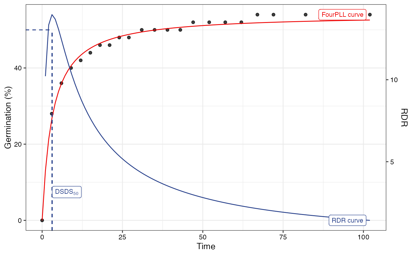
plot(fitL1)
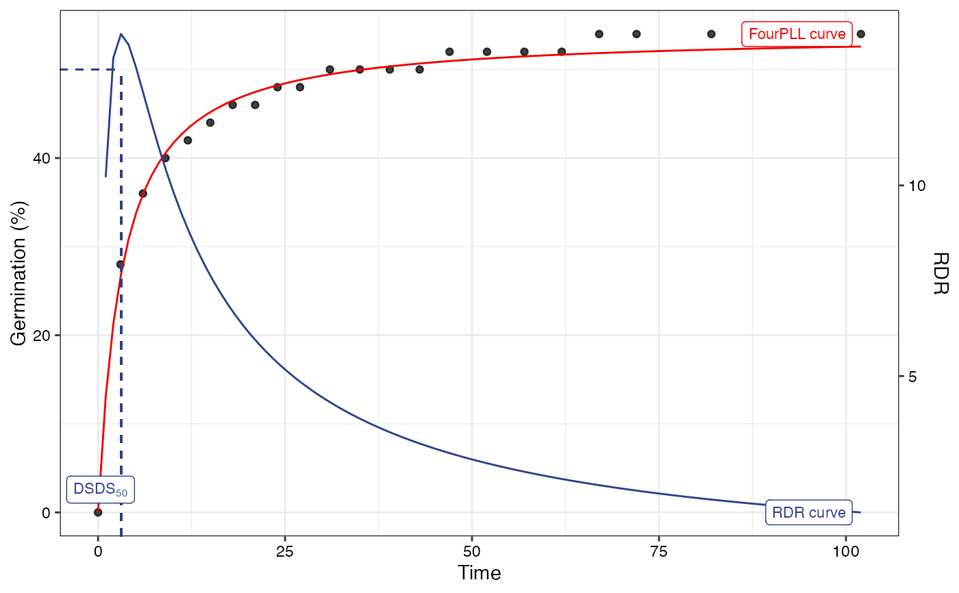
 plot(fitL2)
 # Log-logistic fit
#~~~~~~~~~~~~~~~~~~~~~~~~~~~~~~~~~~~~~~~~~~~~~~~~~~~~~~~~~~~~~~~~~~~~~~~~~~~~
fitLL1 <- FourPLfit(germ.counts = y, intervals = int, rep = rep,
total.seeds = 50, fix.y0 = TRUE, fix.a = TRUE,
inflection.point = "explicit", time.scale = "log")
#> Warning: 'intervals' are not uniform.
fitLL2 <- FourPLfit(germ.counts = y, intervals = int, rep = rep,
total.seeds = 50, fix.y0 = TRUE, fix.a = TRUE,
inflection.point = "implicit", time.scale = "log")
#> Warning: 'intervals' are not uniform.
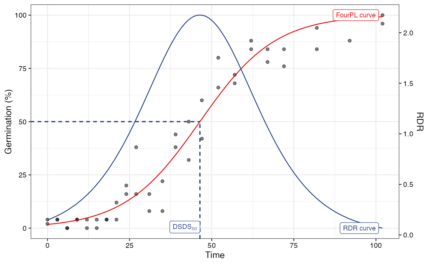
plot(fitLL1)
#> Warning: Removed 1 row containing missing values or values outside the scale range
#> (`geom_function()`).
# Log-logistic fit
#~~~~~~~~~~~~~~~~~~~~~~~~~~~~~~~~~~~~~~~~~~~~~~~~~~~~~~~~~~~~~~~~~~~~~~~~~~~~
fitLL1 <- FourPLfit(germ.counts = y, intervals = int, rep = rep,
total.seeds = 50, fix.y0 = TRUE, fix.a = TRUE,
inflection.point = "explicit", time.scale = "log")
#> Warning: 'intervals' are not uniform.
fitLL2 <- FourPLfit(germ.counts = y, intervals = int, rep = rep,
total.seeds = 50, fix.y0 = TRUE, fix.a = TRUE,
inflection.point = "implicit", time.scale = "log")
#> Warning: 'intervals' are not uniform.
plot(fitLL1)
#> Warning: Removed 1 row containing missing values or values outside the scale range
#> (`geom_function()`).
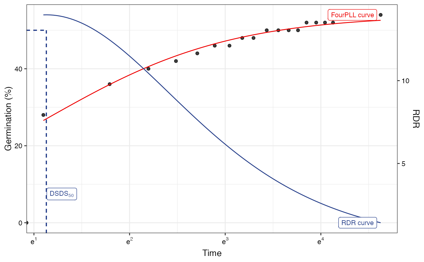
 plot(fitLL1, x.axis.scale = "log")
#> Warning: log-2.718282 transformation introduced infinite values.
#> Warning: log-2.718282 transformation introduced infinite values.
#> Warning: log-2.718282 transformation introduced infinite values.
plot(fitLL1, x.axis.scale = "log")
#> Warning: log-2.718282 transformation introduced infinite values.
#> Warning: log-2.718282 transformation introduced infinite values.
#> Warning: log-2.718282 transformation introduced infinite values.
 plot(fitLL2)
#> Warning: Removed 1 row containing missing values or values outside the scale range
#> (`geom_function()`).
plot(fitLL2)
#> Warning: Removed 1 row containing missing values or values outside the scale range
#> (`geom_function()`).
 plot(fitLL2, x.axis.scale = "log")
#> Warning: log-2.718282 transformation introduced infinite values.
#> Warning: log-2.718282 transformation introduced infinite values.
#> Warning: log-2.718282 transformation introduced infinite values.
plot(fitLL2, x.axis.scale = "log")
#> Warning: log-2.718282 transformation introduced infinite values.
#> Warning: log-2.718282 transformation introduced infinite values.
#> Warning: log-2.718282 transformation introduced infinite values.