Fit seed viability/survival curve to estimate the seed lot constant (Ki) and the period to lose unit probit viability (σ).
FitSigma(data, viability.percent, samp.size, storage.period,
  generalised.model = TRUE, use.cv = FALSE, control.viability = 100)
Arguments
| data | A data frame with the seed viability data recorded periodically. It should possess columns with data on
|
|---|---|
| viability.percent | The name of the column in |
| samp.size | The name of the column in |
| storage.period | The name of the column in |
| generalised.model | logical. If |
| use.cv | logical. If |
| control.viability | The control viability (%). |
Value
A list of class FitSigma with the following components:
A data frame with the data used for computing the model.
The fitted model as an object of class glm (if
generalised.model = TRUE) or lm (if generalised.model = FALSE).
A data.frame of parameter estimates, standard errors and p value.
A one-row data frame with estimates of model fitness such as log likelyhoods, Akaike Information Criterion, Bayesian Information Criterion, deviance and residual degrees of freedom.
The estimated seed lot constant from the model.
The estimated period of time to lose unit probit viability from the model.
Warning or error messages generated during fitting of model, if any.
Details
This function fits seed survival data to the following seed viability equation (Ellis and Roberts 1980) which models the relationship between probit percentage viability and time period of storage.
v = Ki − [ p ⁄ σ ]
or
v = Ki − (1 ⁄ σ)⋅p
Where, v is the probit percentage viability at storage time p (final viability), Ki is the probit percentage viability of the seedlot at the beginning of storage (seedlot constant) and 1⁄σ is the slope.
The above equation may be expressed as a generalized linear model (GLM) with a probit (cumulative normal distribution) link function as follows (Hay et al. 2014) .
y = φ(v) = φ(Ki − (1 ⁄ σ) )
Where, y is the proportion of seeds viabile after time period p and the link function is φ-1, the inverse of the cumulative normal distribution function.
The parameters estimated are the intercept Ki, theoretical viability of the seeds at the start of storage or the seed lot constant, and the slope −σ-1, where σ is the standard deviation of the normal distribution of seed deaths in time or the period of time to lose unit probit viability.
This function can also incorporate a control viability parameter into the model to fit the modified model suggested by (Mead and Gray 1999) . The modified model is as follows.
y = Cv × φ(v) = Cv × φ(Ki − (1 ⁄ σ) )
Where, Cv is the control viability parameter which is the proportion of respondent seeds. This excludes the bias due to seeds of the ageing population that have already lost viability at the start of storage and those non-respondent seeds that are not part of the ageing population due to several reasons.
References
Ellis RH, Roberts EH (1980).
“Improved equations for the prediction of seed longevity.”
Annals of Botany, 45(1), 13--30.
Hay FR, Mead A, Bloomberg M (2014).
“Modelling seed germination in response to continuous variables: use and limitations of probit analysis and alternative approaches.”
Seed Science Research, 24(3), 165--186.
Mead A, Gray D (1999).
“Prediction of seed longevity: A modification of the shape of the Ellis and Roberts seed survival curves.”
Seed Science Research, 9(1), 63--73.
Examples
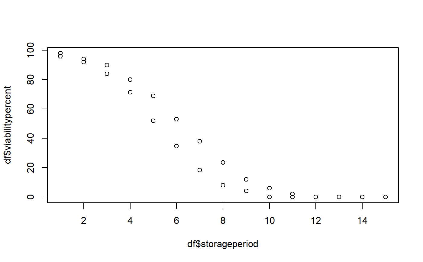
data(seedsurvival) df <- seedsurvival[seedsurvival$crop == "Soybean" & seedsurvival$moistruecontent == 7 & seedsurvival$temperature == 25, c("storageperiod", "rep", "viabilitypercent", "sampsize")] plot(df$storageperiod, df$viabilitypercent)#---------------------------------------------------------------------------- # Generalised linear model with probit link function (without cv) #---------------------------------------------------------------------------- model1a <- FitSigma(data = df, viability.percent = "viabilitypercent", samp.size = "sampsize", storage.period = "storageperiod", generalised.model = TRUE)#>model1a#> Generalised linear model with probit link function. #> Ki Sigma #> 2.373913 2.36206# Raw model model1a$model#> #> Call: glm(formula = frmla, family = binomial(link = "probit"), data = data, #> weights = data$samp.size) #> #> Coefficients: #> (Intercept) storage.period #> 2.3739 -0.4234 #> #> Degrees of Freedom: 29 Total (i.e. Null); 28 Residual #> Null Deviance: 1105 #> Residual Deviance: 27.13 AIC: 100.6# Model parameters model1a$parameters#> term estimate std.error statistic p.value #> 1 Ki 2.3739130 0.12515237 18.96818 3.125234e-80 #> 2 1/sigma -0.4233592 0.01995974 -21.21065 7.614787e-100# Model fit model1a$fit#> null.deviance df.null logLik AIC BIC deviance df.residual #> 1 1104.562 29 -48.30958 100.6192 103.4216 27.13339 28#---------------------------------------------------------------------------- # Generalised linear model with probit link function (with cv) #---------------------------------------------------------------------------- model1b <- FitSigma(data = df, viability.percent = "viabilitypercent", samp.size = "sampsize", storage.period = "storageperiod", generalised.model = TRUE, use.cv = TRUE, control.viability = 98)#>model1b#> Generalised linear model with probit link function. #> Control viability = 98% #> Ki Sigma #> 2.543327 2.252245#># Raw model model1b$model#> #> Call: glm(formula = frmla, family = binomial(link = "probit"), data = data, #> weights = data$samp.size) #> #> Coefficients: #> (Intercept) storage.period #> 2.543 -0.444 #> #> Degrees of Freedom: 29 Total (i.e. Null); 28 Residual #> Null Deviance: 1153 #> Residual Deviance: 29.12 AIC: 99.11# Model parameters model1b$parameters#> term estimate std.error statistic p.value #> 1 Ki 2.5433272 0.13274622 19.15932 8.092372e-82 #> 2 1/sigma -0.4440014 0.02104155 -21.10117 7.758893e-99# Model fit model1b$fit#> null.deviance df.null logLik AIC BIC deviance df.residual #> 1 1153.011 29 -47.55712 99.11424 101.9166 29.12018 28#---------------------------------------------------------------------------- # Linear model after probit transformation (without cv) #---------------------------------------------------------------------------- model2a <- FitSigma(data = df, viability.percent = "viabilitypercent", samp.size = "sampsize", storage.period = "storageperiod", generalised.model = FALSE)#>model2a#> Linear model after probit transformation. #> Ki Sigma #> 2.014134 2.810871# Raw model model2a$model#> #> Call: #> lm(formula = frmla, data = data) #> #> Coefficients: #> (Intercept) storage.period #> 2.0141 -0.3558 #># Model parameters model2a$parameters#> term estimate std.error statistic p.value #> 1 Ki 2.0141338 0.15709049 12.82149 3.074991e-13 #> 2 1/sigma -0.3557616 0.01727765 -20.59086 1.887632e-18# Model fit model2a$fit#> r.squared adj.r.squared sigma statistic p.value df logLik #> 1 0.9380508 0.9358384 0.4088638 423.9834 1.887632e-18 2 -14.70207 #> AIC BIC deviance df.residual #> 1 35.40414 39.60773 4.68075 28#---------------------------------------------------------------------------- # Linear model after probit transformation (with cv) #---------------------------------------------------------------------------- model2b <- FitSigma(data = df, viability.percent = "viabilitypercent", samp.size = "sampsize", storage.period = "storageperiod", generalised.model = FALSE, use.cv = TRUE, control.viability = 98)#>model2b#> Linear model after probit transformation. #> Control viability = 98% #> Ki Sigma #> 2.055239 2.754653# Raw model model2b$model#> #> Call: #> lm(formula = frmla, data = data) #> #> Coefficients: #> (Intercept) storage.period #> 2.055 -0.363 #># Model parameters model2b$parameters#> term estimate std.error statistic p.value #> 1 Ki 2.0552385 0.16029642 12.82149 3.074991e-13 #> 2 1/sigma -0.3630221 0.01763026 -20.59086 1.887632e-18# Model fit model2b$fit#> r.squared adj.r.squared sigma statistic p.value df logLik AIC #> 1 0.9380508 0.9358384 0.417208 423.9834 1.887632e-18 2 -15.30815 36.6163 #> BIC deviance df.residual #> 1 40.81989 4.87375 28