Box Plots

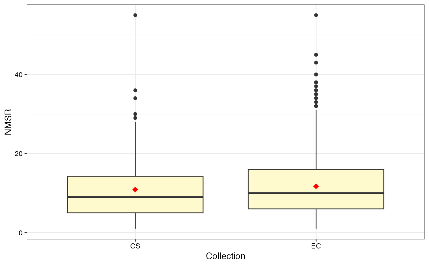
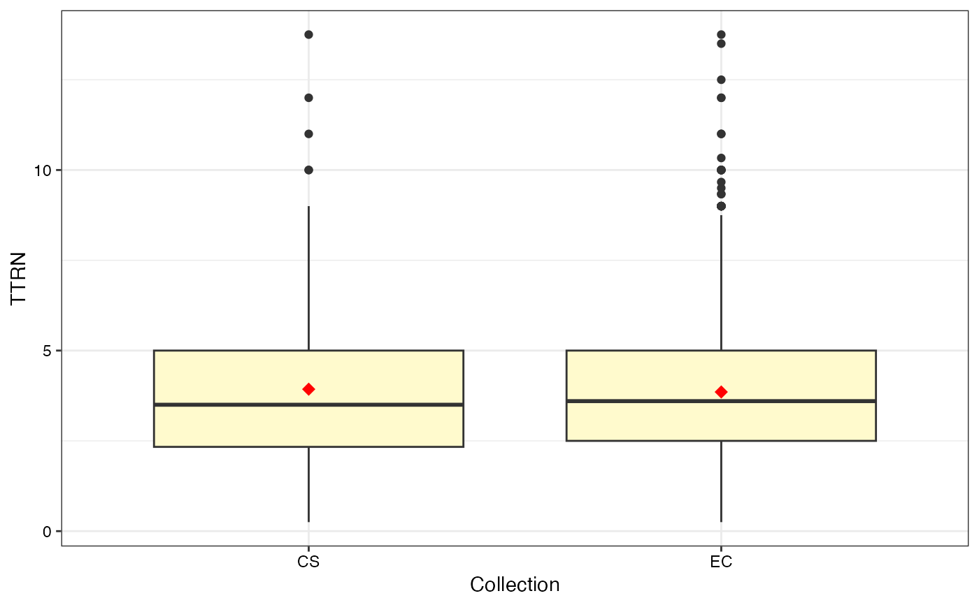
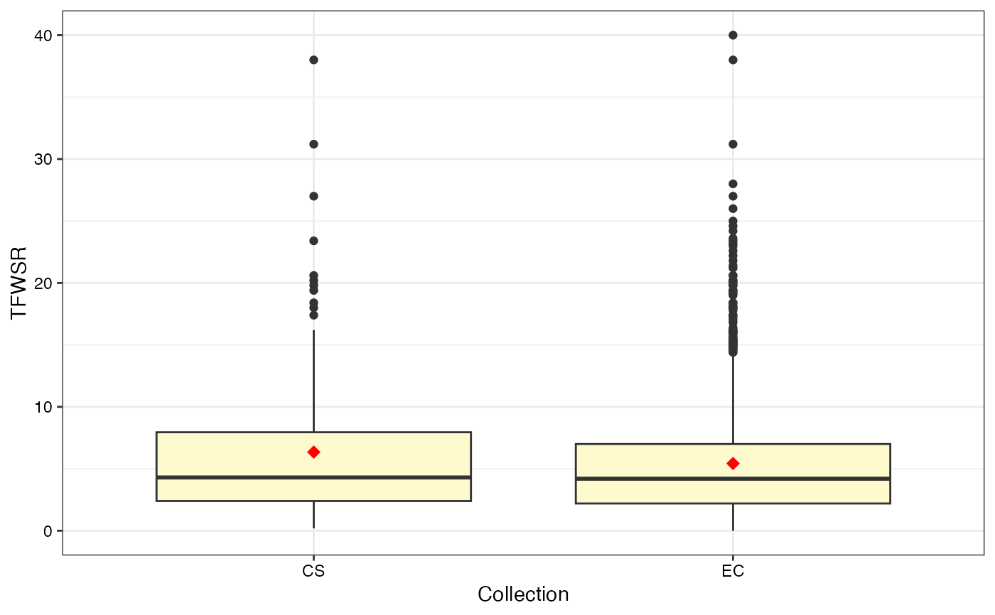
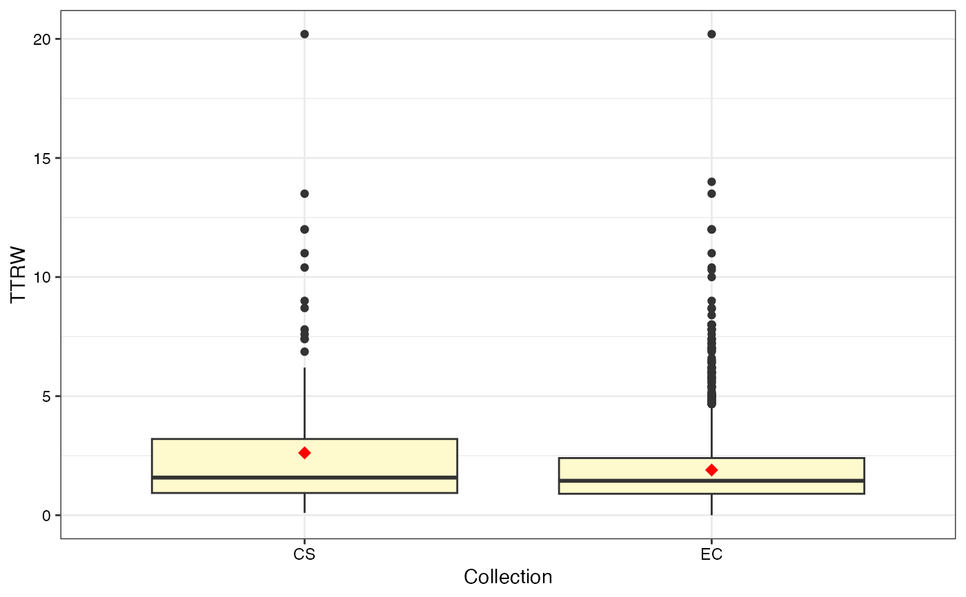
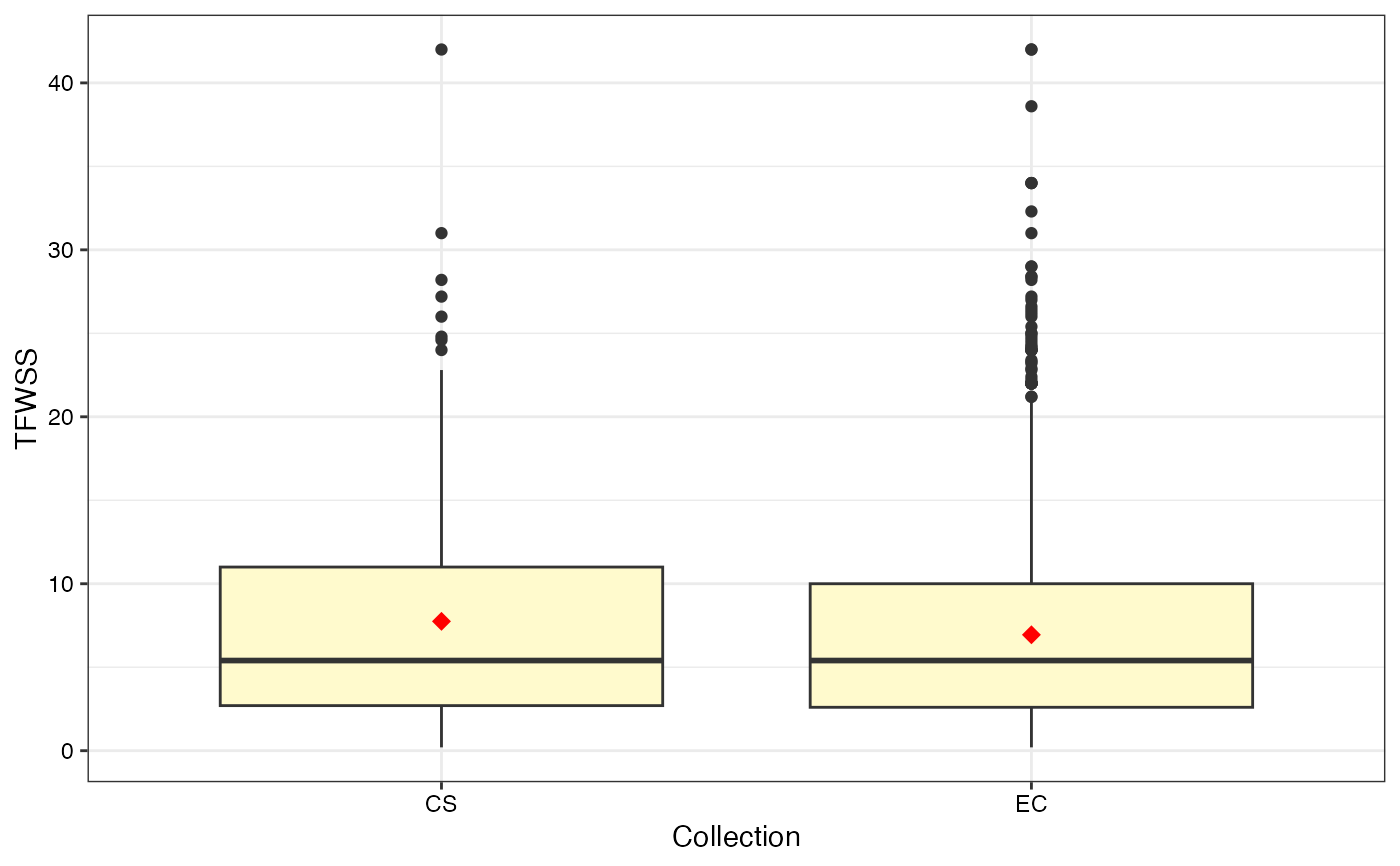
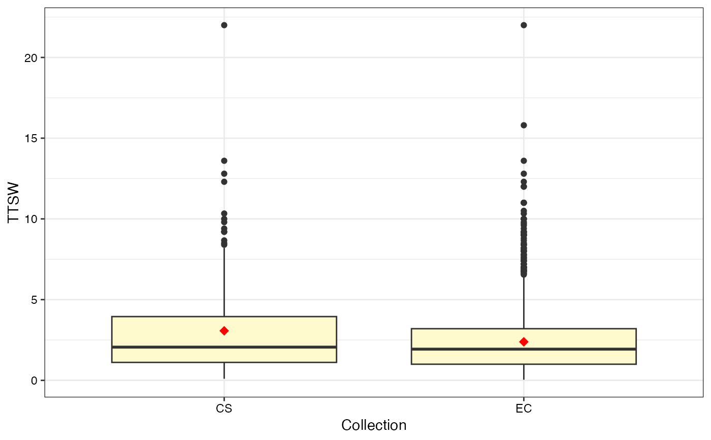
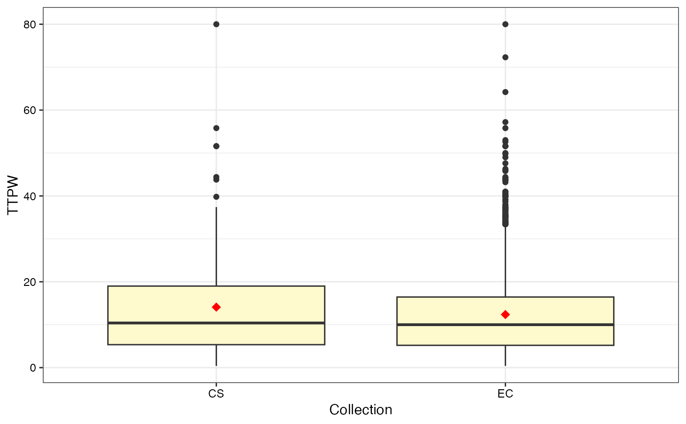
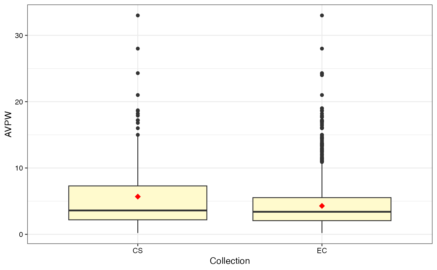
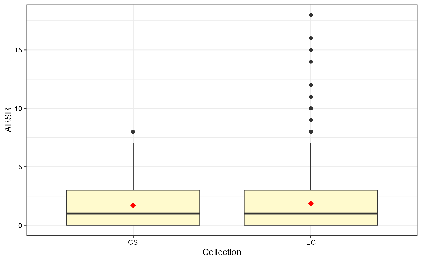
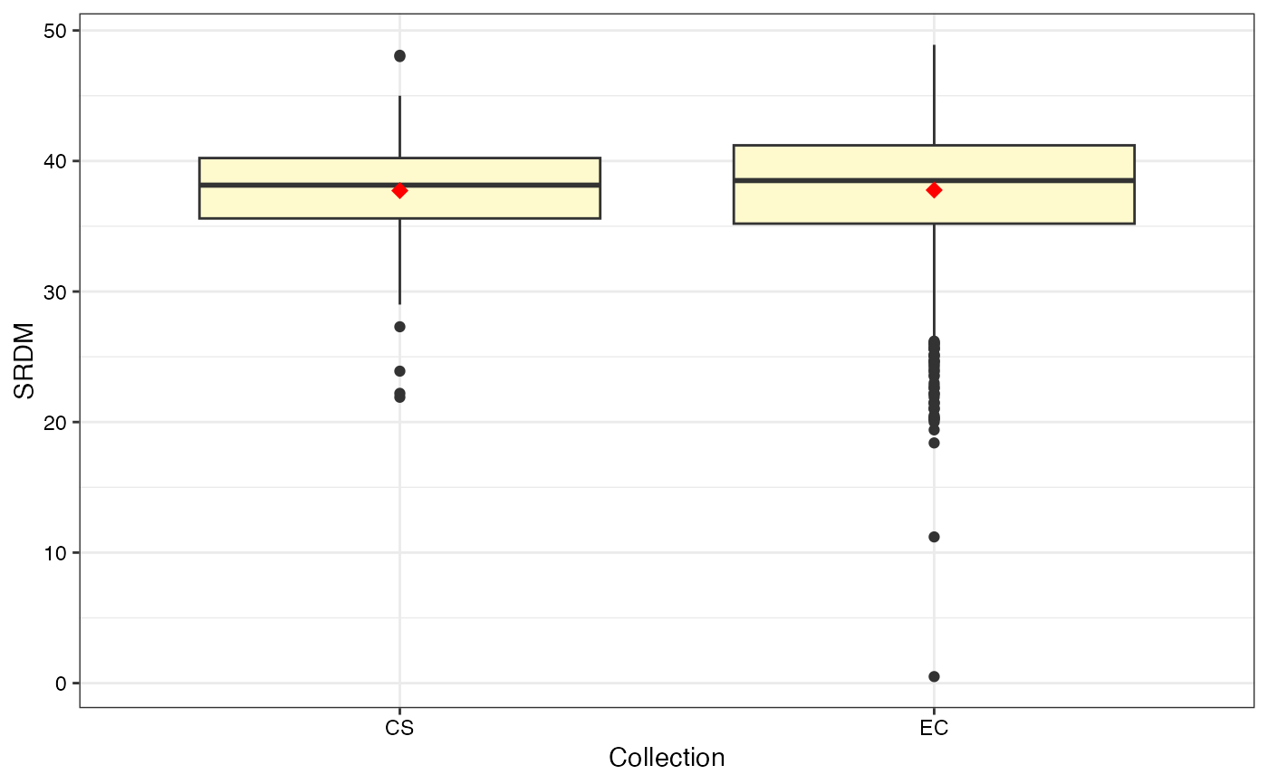
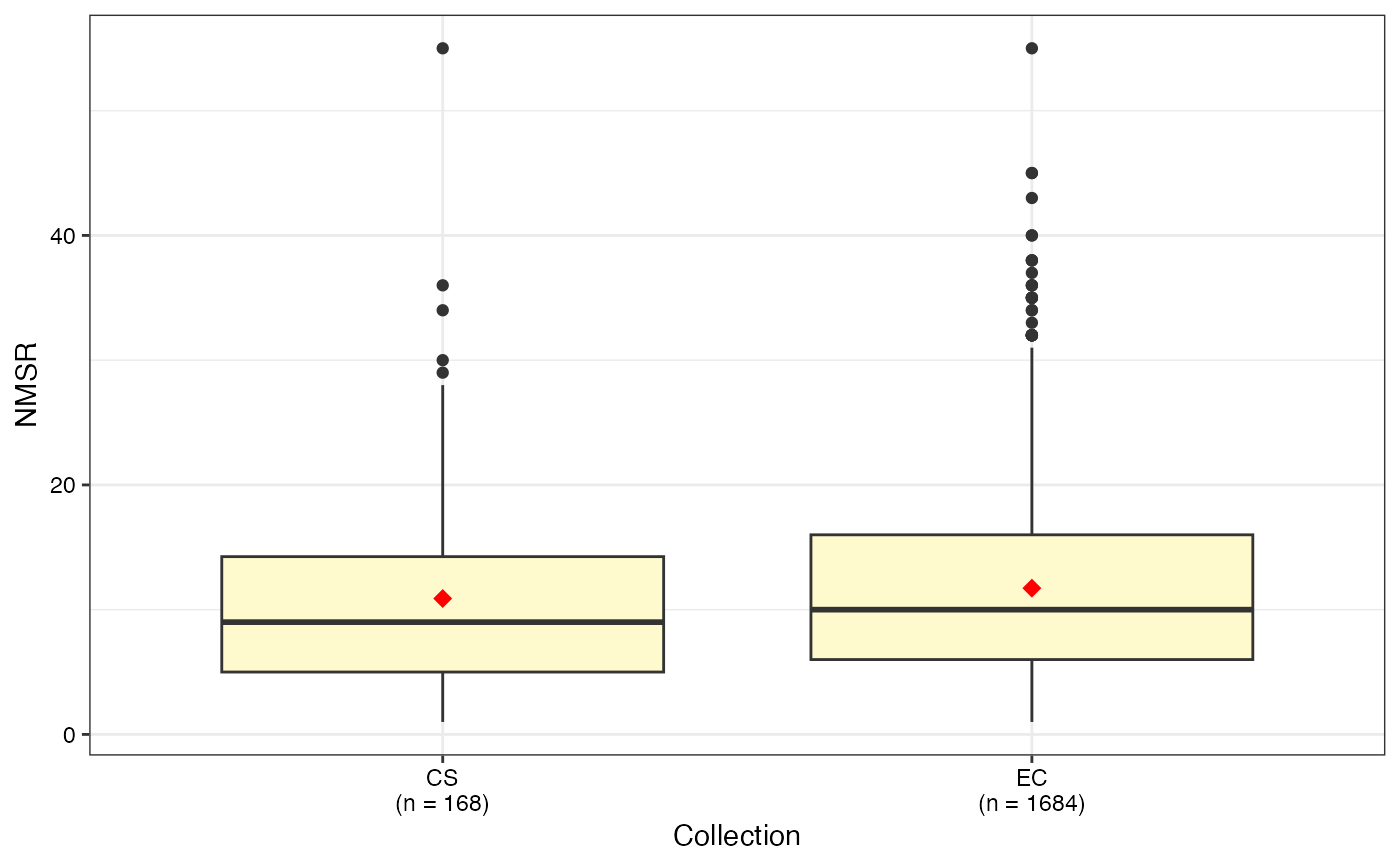
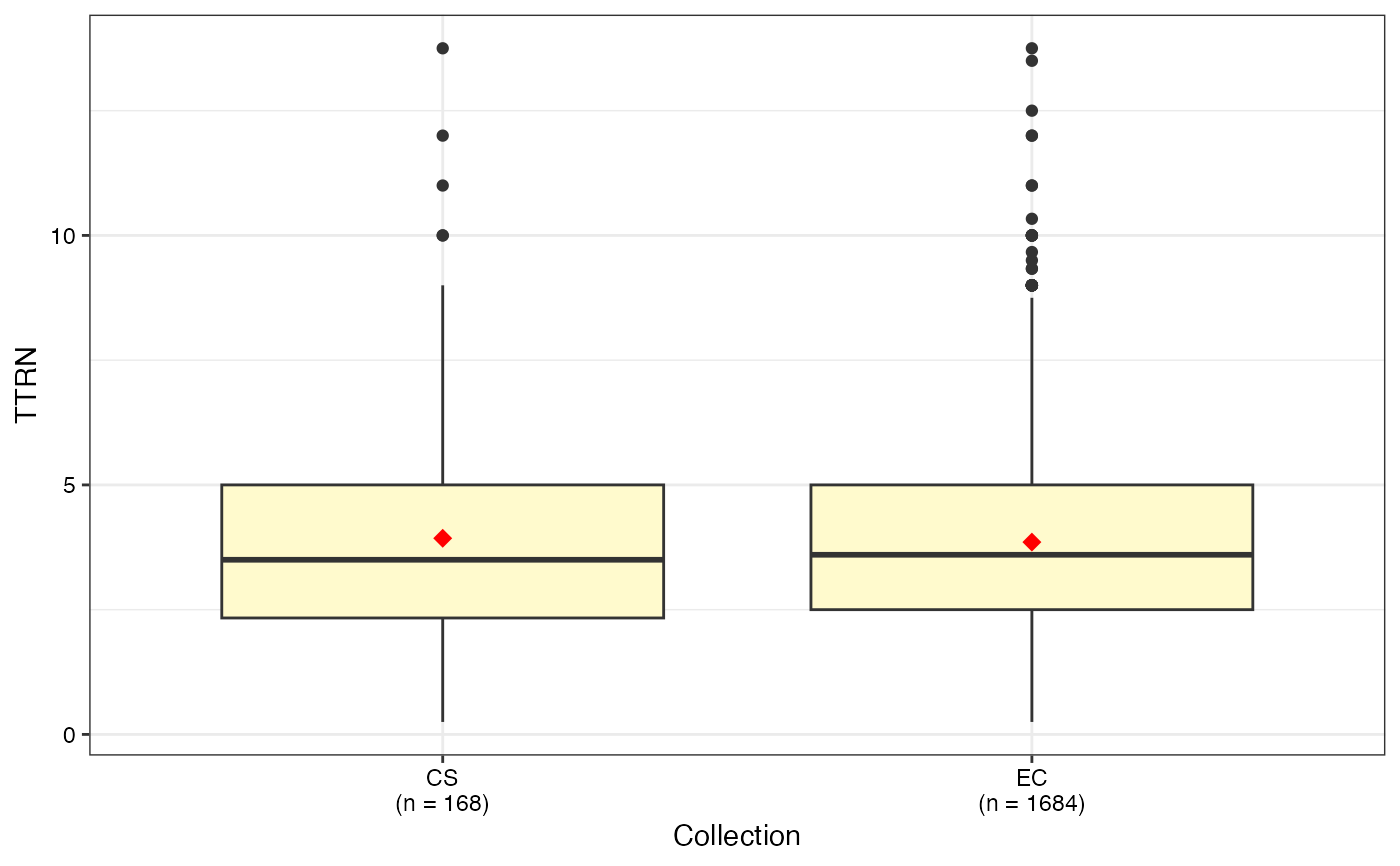
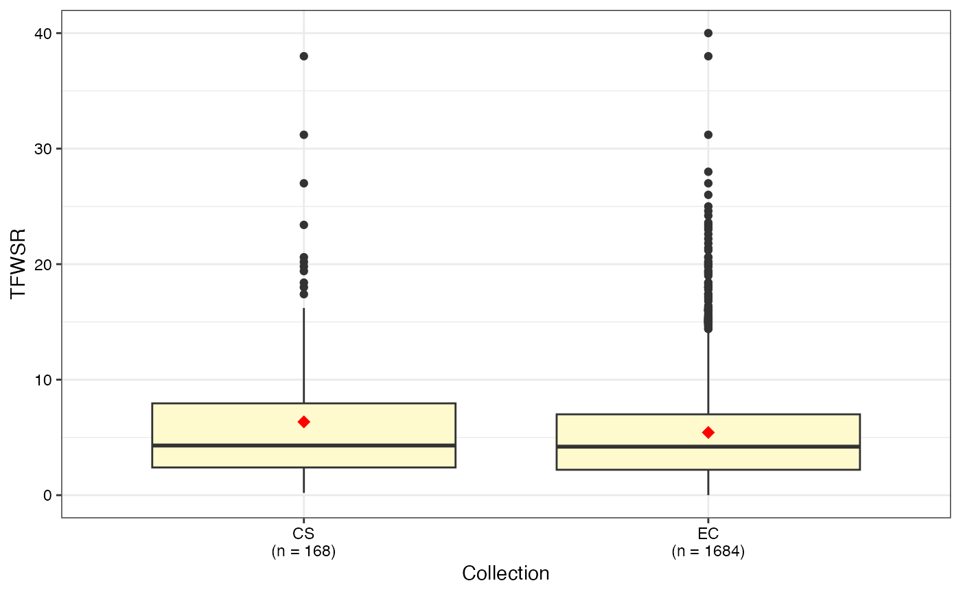
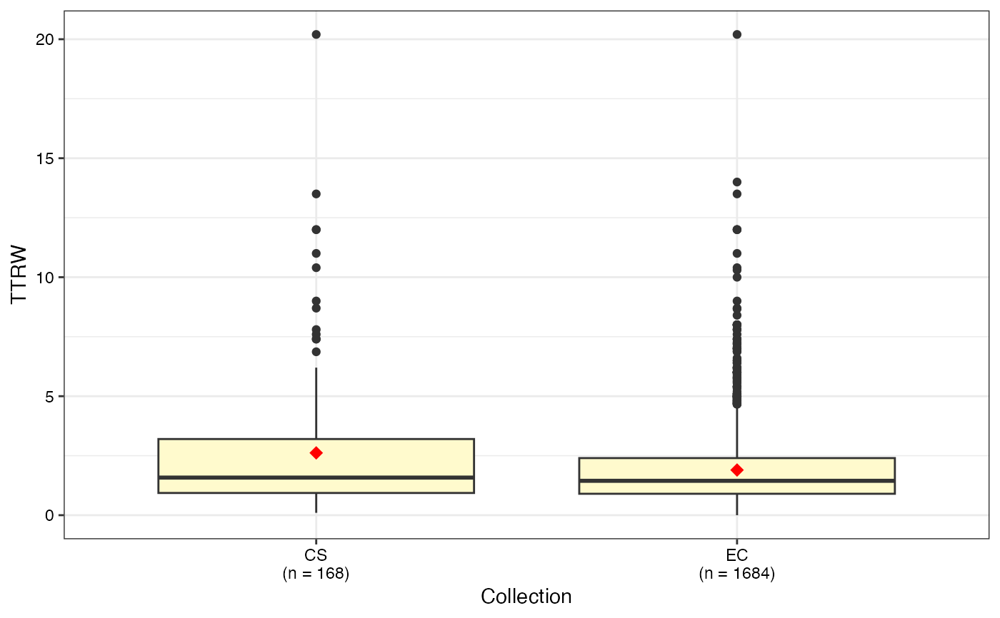
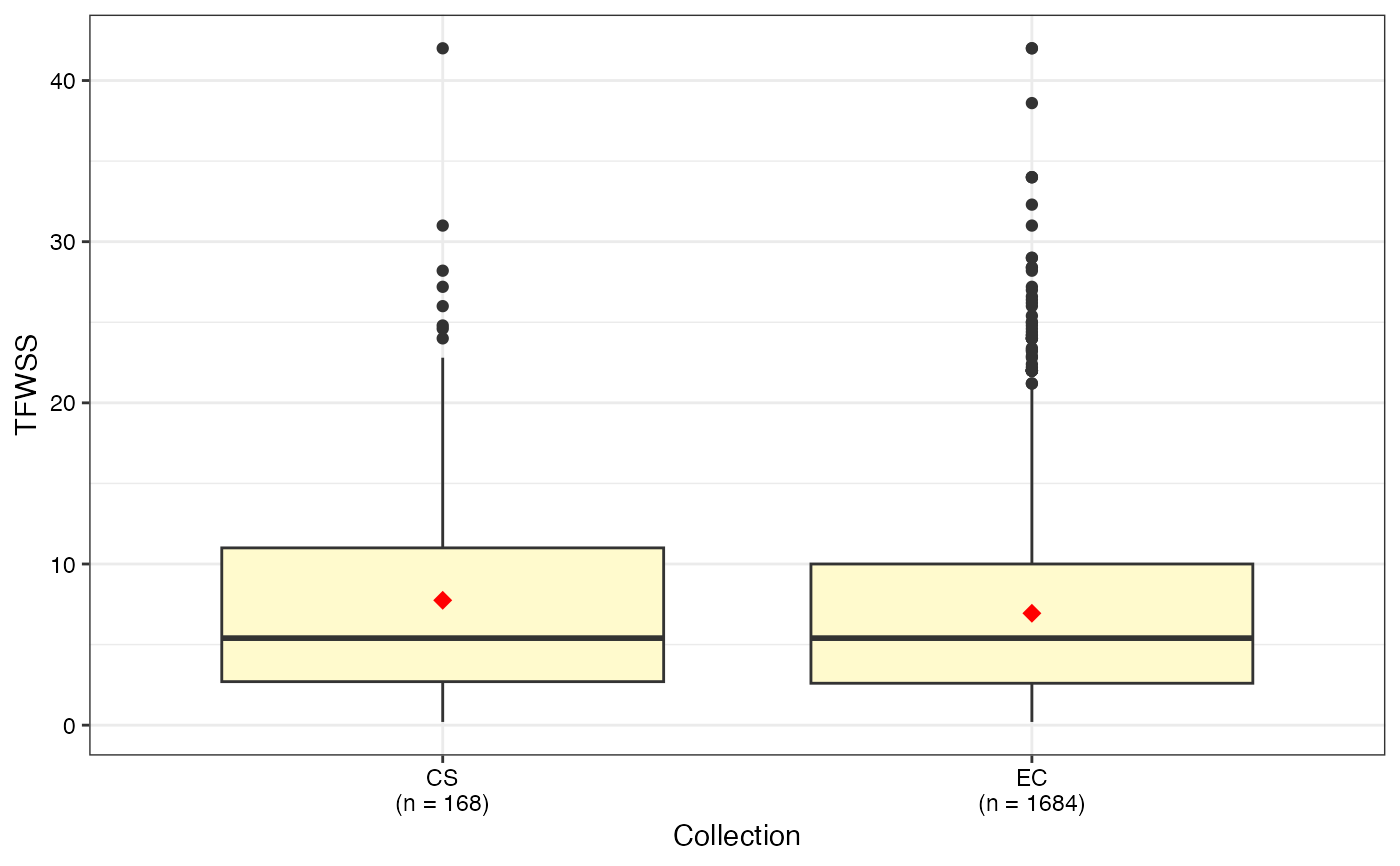
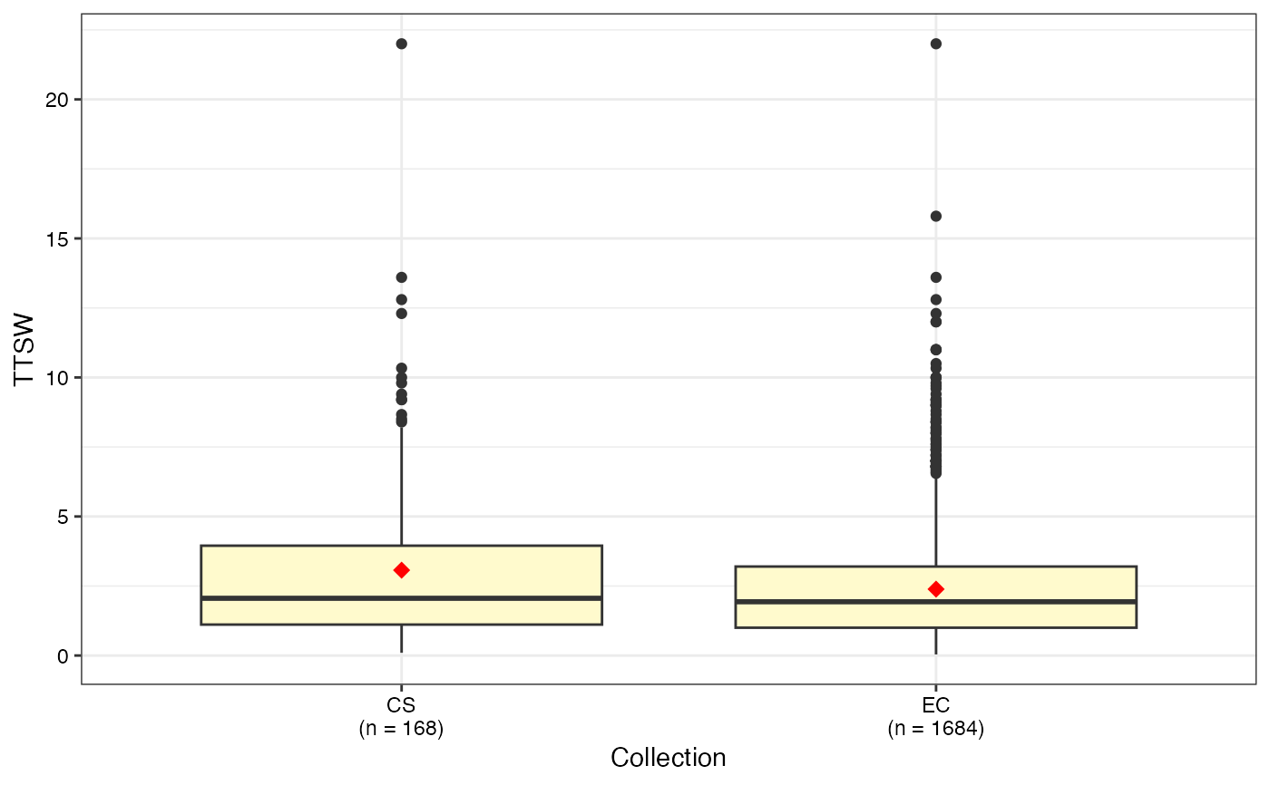
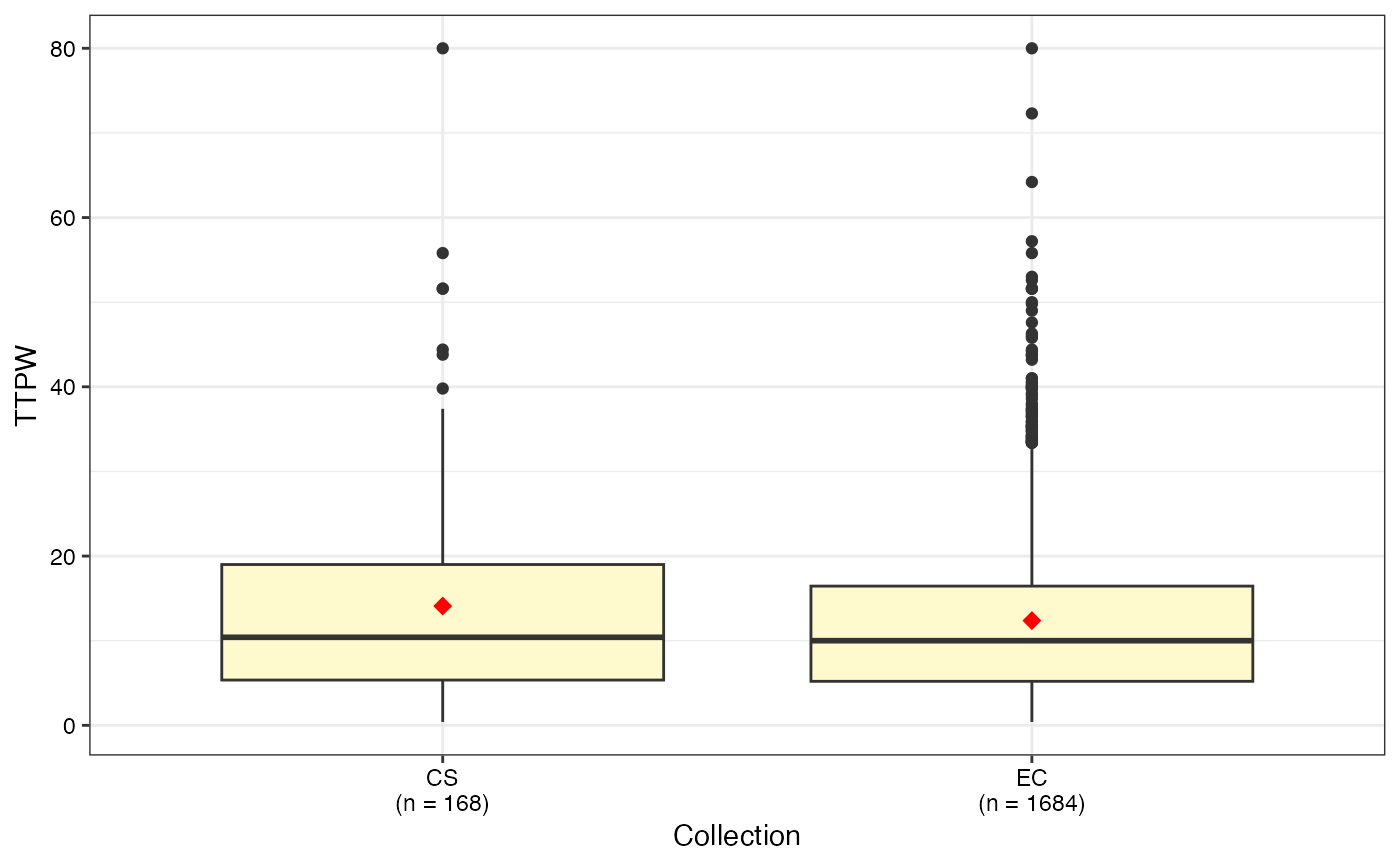
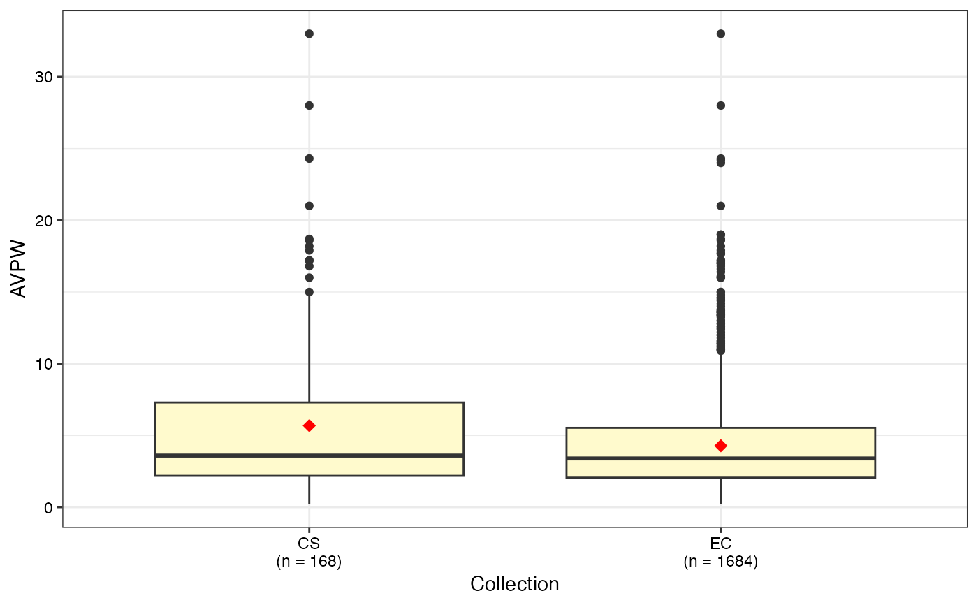
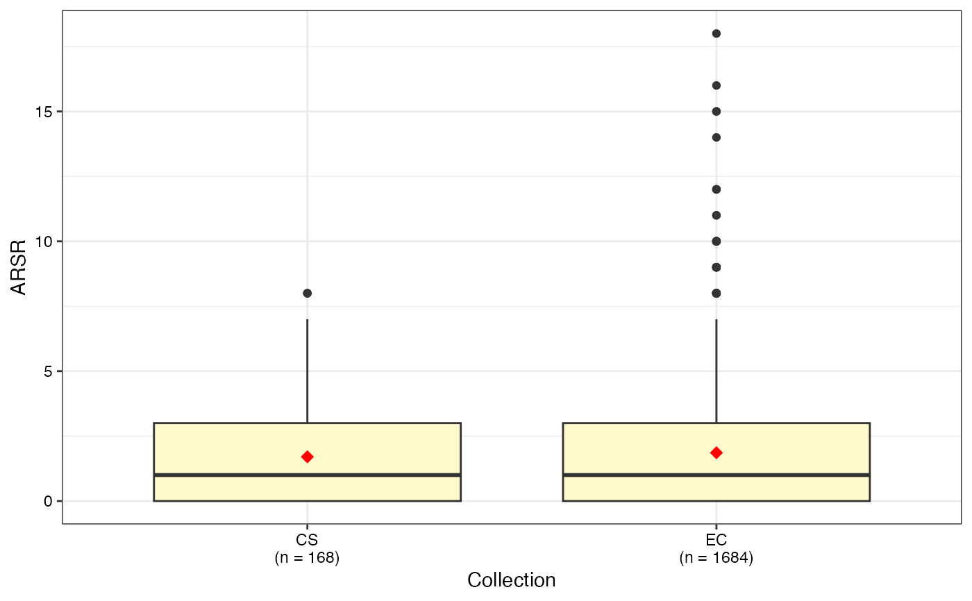
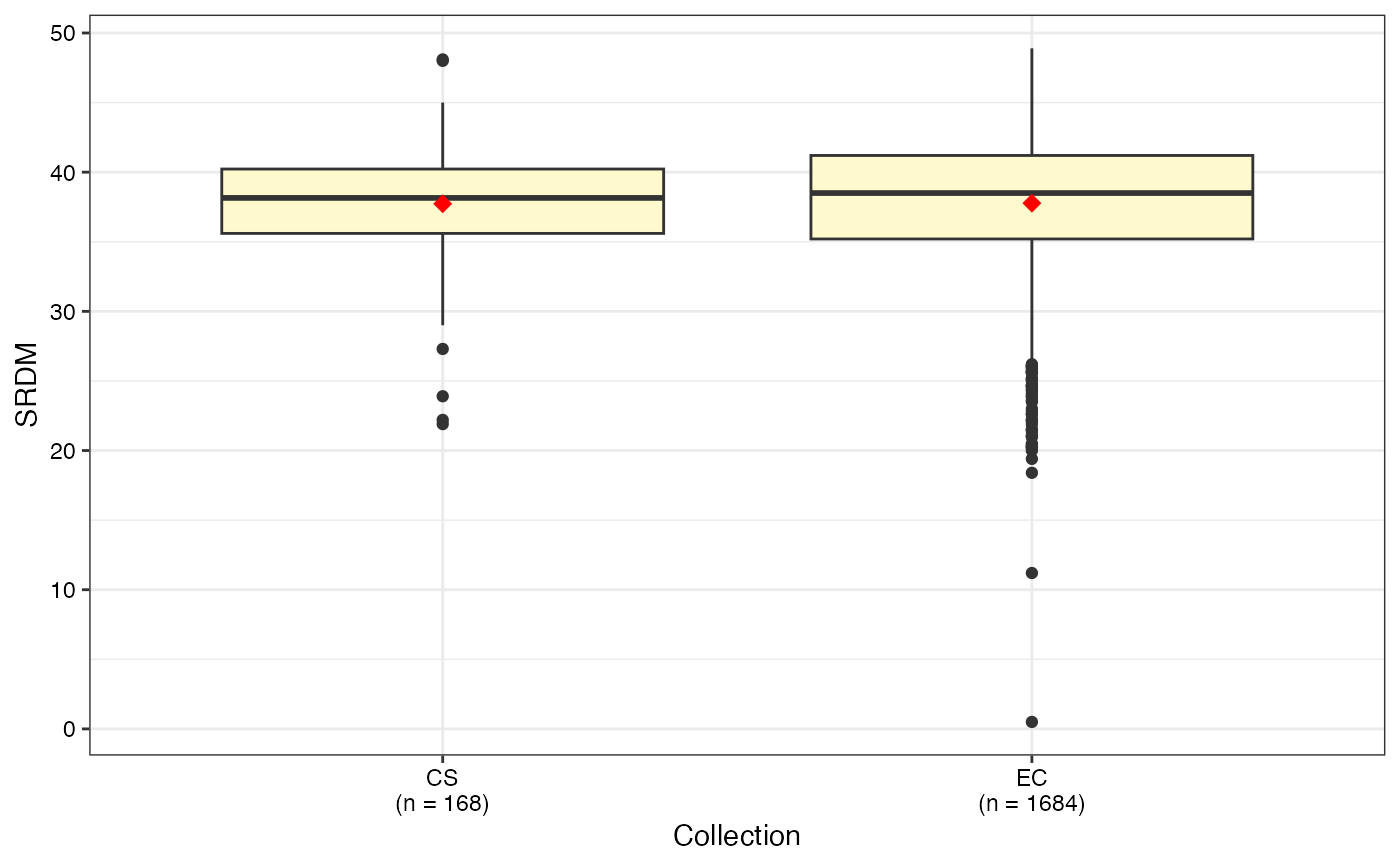
Plot Box-and-Whisker plots (Tukey 1970; McGill et al. 1978) to graphically compare the probability distributions of quantitative traits between entire collection (EC) and core set (CS).

box.evaluate.core(data, names, quantitative, selected)

Arguments

data: The data as a data frame object. The data frame should possess one row per individual and columns with the individual names and multiple trait/character data.
names: Name of column with the individual names as a character string
quantitative: Name of columns with the quantitative traits as a character vector.
selected: Character vector with the names of individuals selected in core collection and present in the names column.

Value

A list with the ggplot objects of box plots of CS and EC for each trait specified as quantitative.

References

McGill R, Tukey JW, Larsen WA (1978). “Variations of box plots.” The American Statistician, 32(1), 12.

Tukey JW (1970). Exploratory Data Analysis. Preliminary edition. Addison-Wesley.

Examples


data("cassava_CC")
data("cassava_EC")

ec <- cbind(genotypes = rownames(cassava_EC), cassava_EC)
ec$genotypes <- as.character(ec$genotypes)
rownames(ec) <- NULL

core <- rownames(cassava_CC)

quant <- c("NMSR", "TTRN", "TFWSR", "TTRW", "TFWSS", "TTSW", "TTPW", "AVPW",
           "ARSR", "SRDM")
qual <- c("CUAL", "LNGS", "PTLC", "DSTA", "LFRT", "LBTEF", "CBTR", "NMLB",
          "ANGB", "CUAL9M", "LVC9M", "TNPR9M", "PL9M", "STRP", "STRC",
          "PSTR")

ec[, qual] <- lapply(ec[, qual],
                     function(x) factor(as.factor(x)))

box.evaluate.core(data = ec, names = "genotypes",
                  quantitative = quant, selected = core)
#> $NMSR

#> 
#> $TTRN

#> 
#> $TFWSR

#> 
#> $TTRW

#> 
#> $TFWSS

#> 
#> $TTSW

#> 
#> $TTPW

#> 
#> $AVPW

#> 
#> $ARSR

#> 
#> $SRDM

#>

Arguments

Value

References

See also

Examples