Compute phenotypic correlations (Pearson 1895) between traits, plot correlation matrices as correlograms (Friendly 2002) and calculate mantel correlation (Legendre and Legendre 2012) between them to compare entire collection (EC) and core set (CS).
Arguments
- data
The data as a data frame object. The data frame should possess one row per individual and columns with the individual names and multiple trait/character data.
- names
Name of column with the individual names as a character string.
- quantitative
Name of columns with the quantitative traits as a character vector.
- qualitative
Name of columns with the qualitative traits as a character vector.
- selected
Character vector with the names of individuals selected in core collection and present in the
namescolumn.
Value
A list with the following components.
- Correlation Matrix
The matrix with phenotypic correlations between traits in EC (below diagonal) and CS (above diagonal).
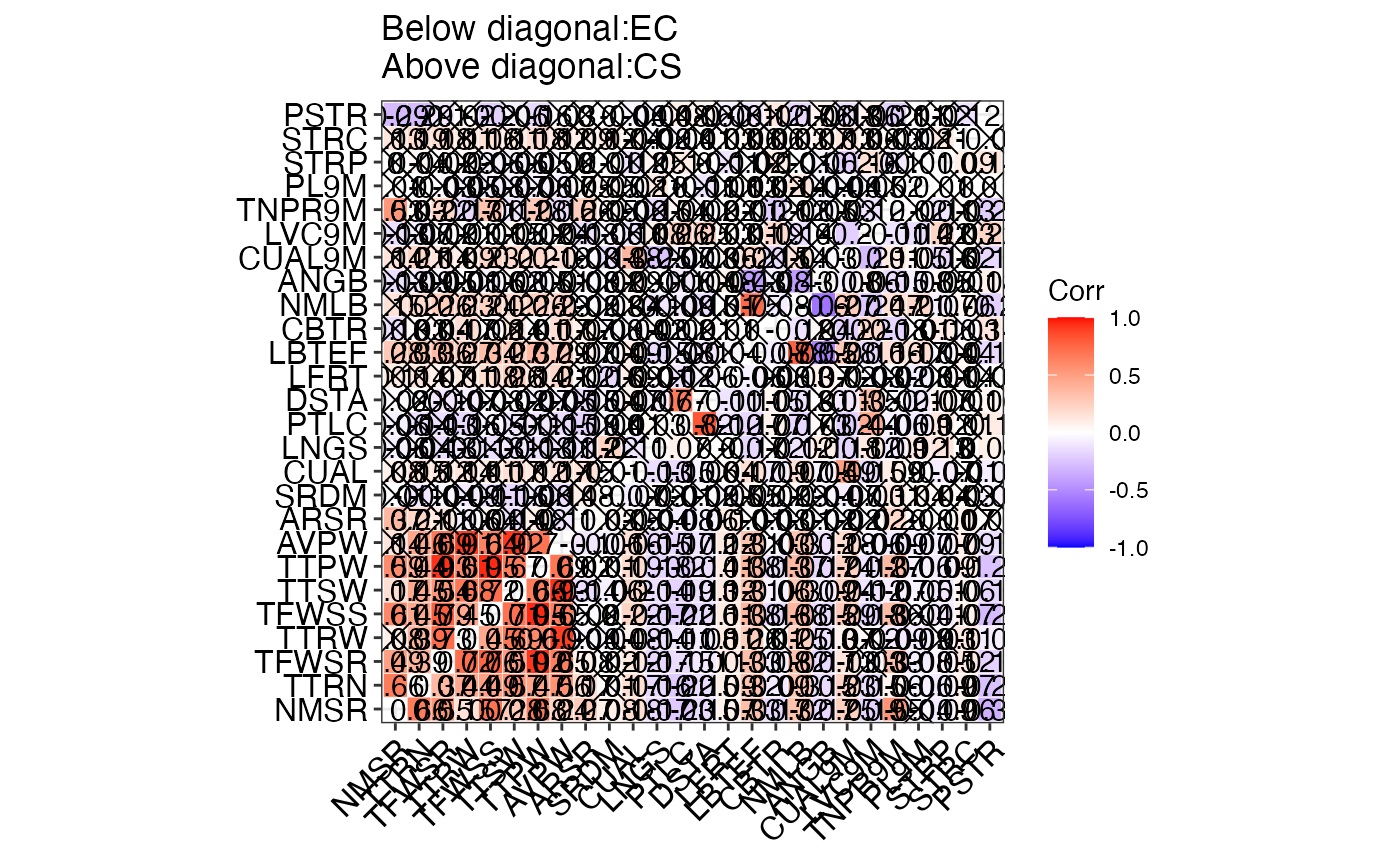
- Correologram
A correlogram of phenotypic correlations between traits in EC (below diagonal) and CS (above diagonal) as a
ggplotobject.- Mantel Correlation
A data frame with Mantel correlation coefficient (\(r\)) between EC and CS phenotypic correlation matrices, it's p value and significance (*: p \(\leq\) 0.01; **: p \(\leq\) 0.05; ns: p \( > \) 0.05).
References
Friendly M (2002).
“Corrgrams.”
The American Statistician, 56(4), 316–324.
Legendre P, Legendre L (2012).
“Interpretation of ecological structures.”
In Developments in Environmental Modelling, volume 24, 521–624.
Elsevier.
Pearson K (1895).
“Note on regression and inheritance in the case of two parents.”
Proceedings of the Royal Society of London, 58, 240–242.
Examples
data("cassava_CC")
data("cassava_EC")

ec <- cbind(genotypes = rownames(cassava_EC), cassava_EC)
ec$genotypes <- as.character(ec$genotypes)
rownames(ec) <- NULL

core <- rownames(cassava_CC)

quant <- c("NMSR", "TTRN", "TFWSR", "TTRW", "TFWSS", "TTSW", "TTPW", "AVPW",
           "ARSR", "SRDM")
qual <- c("CUAL", "LNGS", "PTLC", "DSTA", "LFRT", "LBTEF", "CBTR", "NMLB",
          "ANGB", "CUAL9M", "LVC9M", "TNPR9M", "PL9M", "STRP", "STRC",
          "PSTR")

ec[, qual] <- lapply(ec[, qual],
                     function(x) factor(as.factor(x)))

corr.evaluate.core(data = ec, names = "genotypes", quantitative = quant,
                   qualitative = qual, selected = core)
#> Warning: `aes_string()` was deprecated in ggplot2 3.0.0.
#> ℹ Please use tidy evaluation idioms with `aes()`.
#> ℹ See also `vignette("ggplot2-in-packages")` for more information.
#> ℹ The deprecated feature was likely used in the ggcorrplot package.
#>   Please report the issue at <https://github.com/kassambara/ggcorrplot/issues>.
#> $`Correlation Matrix`
#>           NMSR    TTRN   TFWSR    TTRW   TFWSS    TTSW    TTPW    AVPW    ARSR
#> NMSR      <NA>  0.66**  0.49**    0.08  0.61**   0.17*  0.59**    0.14  0.37**
#> TTRN    0.66**    <NA>  0.39**  0.39**  0.45**  0.45**  0.44**  0.46**  0.21**
#> TFWSR   0.55**  0.37**    <NA>  0.73**  0.79**  0.54**  0.93**  0.69**    0.11
#> TTRW    0.15**  0.44**  0.72**    <NA>  0.45**  0.68**  0.61**  0.91**   -0.06
#> TFWSS   0.70**  0.49**  0.76**  0.45**    <NA>  0.72**  0.95**  0.64**    0.04
#> TTSW    0.28**  0.57**  0.51**  0.69**  0.71**    <NA>  0.67**  0.92**   -0.14
#> TTPW    0.68**  0.47**  0.92**  0.60**  0.95**  0.66**    <NA>  0.70**    0.08
#> AVPW    0.24**  0.56**  0.65**  0.90**  0.65**  0.93**  0.69**    <NA>   -0.11
#> ARSR    0.27**  0.17**  0.08**   -0.04   -0.02 -0.14**    0.02 -0.10**    <NA>
#> SRDM    0.08**    0.01    0.02   -0.04    0.00  -0.06*    0.01  -0.06*    0.03
#> CUAL    0.18**  0.17**  0.12**  0.08**  0.22**  0.20**  0.19**  0.16**    0.05
#> LNGS   -0.17** -0.16** -0.17** -0.14** -0.17** -0.14** -0.18** -0.15**   -0.04
#> PTLC   -0.23** -0.22** -0.15** -0.11** -0.22** -0.19** -0.20** -0.17** -0.08**
#> DSTA   -0.15** -0.15** -0.10** -0.08** -0.16** -0.13** -0.14** -0.12**  -0.06*
#> LFRT    0.07**  0.09**  0.10**  0.11**  0.11**  0.12**  0.11**  0.12**  0.10**
#> LBTEF   0.33**  0.32**  0.33**  0.26**  0.38**  0.31**  0.38**  0.31**   -0.01
#> CBTR   -0.17** -0.09** -0.08**    0.01 -0.16** -0.06** -0.13**   -0.03   -0.03
#> NMLB    0.32**  0.30**  0.32**  0.25**  0.38**  0.30**  0.37**  0.30**   -0.01
#> ANGB   -0.17** -0.15** -0.17** -0.13** -0.15** -0.09** -0.17** -0.12**   -0.02
#> CUAL9M  0.25**  0.23**  0.13**  0.07**  0.29**  0.24**  0.24**  0.18**   -0.02
#> LVC9M  -0.19** -0.15**   -0.03    0.02 -0.18** -0.12** -0.12**  -0.06*   -0.02
#> TNPR9M  0.55**   0.06*  0.33** -0.09**  0.36** -0.07**  0.37** -0.09**  0.20**
#> PL9M     -0.04  -0.06* -0.08** -0.09**   -0.04  -0.05*  -0.06* -0.07**   -0.00
#> STRP   -0.09** -0.09**  -0.05*   -0.03 -0.10** -0.10** -0.09** -0.07**   -0.01
#> STRC     0.06*  0.07**  0.12**  0.11**  0.07**   0.06*  0.10**  0.09**  0.07**
#> PSTR   -0.34** -0.27** -0.19** -0.07** -0.29** -0.18** -0.26** -0.14**    0.01
#>           SRDM    CUAL    LNGS    PTLC    DSTA    LFRT   LBTEF    CBTR    NMLB
#> NMSR     -0.01    0.08   -0.06   -0.06   -0.02    0.10  0.28**   -0.13    0.15
#> TTRN     -0.10    0.15   -0.04   -0.14   -0.00    0.14  0.33**    0.03  0.20**
#> TFWSR    -0.04    0.12   -0.13   -0.13   -0.10    0.07  0.36**    0.04  0.26**
#> TTRW     -0.09    0.14   -0.10  -0.16*   -0.07    0.11  0.27**   0.17*  0.23**
#> TFWSS    -0.11    0.11   -0.13   -0.05   -0.03   0.18*  0.34**   -0.02  0.24**
#> TTSW    -0.16*   0.17*   -0.10   -0.11   -0.02  0.26**  0.27**    0.14  0.20**
#> TTPW     -0.08    0.12   -0.13   -0.10   -0.07    0.14  0.37**    0.01  0.26**
#> AVPW     -0.14   0.17*   -0.11   -0.15   -0.05  0.21**  0.29**   0.17*  0.23**
#> ARSR      0.08    0.15   -0.12  -0.19*   -0.15    0.02    0.07    0.07   -0.02
#> SRDM      <NA>   -0.01  0.22**   -0.04   -0.04  -0.16*   -0.04   -0.03   -0.03
#> CUAL   -0.07**    <NA>   -0.11    0.01    0.07    0.09    0.09   -0.04    0.04
#> LNGS      0.03 -0.13**    <NA>    0.03   -0.07   -0.01  -0.15*    0.02   -0.10
#> PTLC     -0.01 -0.15**  0.07**    <NA>  0.67**   -0.12   -0.08   -0.02   -0.09
#> DSTA     -0.02  -0.06*    0.00  0.82**    <NA>   -0.06   -0.10    0.01   -0.15
#> LFRT     -0.05    0.04   -0.00 -0.12** -0.11**    <NA>   -0.04    0.01    0.01
#> LBTEF     0.05  0.17** -0.17** -0.17** -0.11**  -0.06*    <NA>    0.00  0.75**
#> CBTR     -0.02 -0.09**    0.02  0.07**   0.05*   -0.03 -0.08**    <NA>   -0.08
#> NMLB      0.03  0.17** -0.12** -0.17** -0.13**   -0.03  0.78** -0.12**    <NA>
#> ANGB     -0.04  -0.05*  0.10**    0.03    0.01  0.07** -0.55**    0.04 -0.60**
#> CUAL9M -0.07**  0.49** -0.18** -0.20** -0.10**    0.02  0.28** -0.20**  0.27**
#> LVC9M    -0.03 -0.15**  0.12**  0.44**  0.35**   -0.03 -0.16**  0.20** -0.24**
#> TNPR9M  0.11**  0.09** -0.09**  -0.06*   -0.02   -0.02  0.16** -0.18**  0.17**
#> PL9M      0.04   -0.00  0.12** -0.09** -0.10** -0.08**  0.17**   -0.01  0.21**
#> STRP      0.04 -0.07**  0.13**  0.12**  0.07**   -0.01   -0.04  0.10** -0.07**
#> STRC      0.03   -0.01    0.00    0.01   -0.01    0.04    0.04   -0.03   0.06*
#> PSTR     -0.05 -0.08**  0.08**  0.10**  0.06**   -0.01 -0.16**  0.14** -0.20**
#>           ANGB  CUAL9M   LVC9M  TNPR9M  PL9M    STRP  STRC    PSTR
#> NMSR     -0.13    0.14   -0.13  0.53**  0.01    0.00  0.13 -0.29**
#> TTRN     -0.09  0.21**   -0.07    0.03 -0.00    0.04 0.19* -0.29**
#> TFWSR    -0.05    0.14   -0.02  0.22** -0.03   -0.02 0.18*   -0.10
#> TTRW     -0.01    0.09    0.01  -0.17* -0.05    0.03  0.11    0.02
#> TFWSS    -0.06  0.23**   -0.01  0.31** -0.08   -0.06 0.16*  -0.20*
#> TTSW      0.02   0.20*    0.05   -0.11 -0.07   -0.06  0.11   -0.06
#> TTPW     -0.05  0.20**   -0.02  0.28** -0.06   -0.05 0.18*  -0.16*
#> AVPW      0.01   0.16*    0.04  -0.15* -0.07   -0.02  0.12   -0.03
#> ARSR     -0.03   -0.03   -0.13  0.26**  0.05   -0.00  0.09   -0.00
#> SRDM     -0.02   -0.14   -0.05    0.05  0.05    0.01  0.12    0.00
#> CUAL      0.09  0.38**   -0.11   -0.02 -0.02   -0.12  0.04   -0.04
#> LNGS     -0.01 -0.25**    0.08   -0.15  0.11    0.05 -0.02   -0.04
#> PTLC     -0.10   -0.07  0.26**    0.04  0.00    0.10 -0.04    0.08
#> DSTA     -0.04   -0.03  0.25**   -0.02 -0.11    0.00  0.01    0.06
#> LFRT      0.08    0.06    0.03    0.02 -0.01   -0.11  0.03   -0.08
#> LBTEF  -0.43**  0.20**    0.01    0.01  0.03   -0.02  0.06   -0.10
#> CBTR     -0.08   -0.15   0.19* -0.21**  0.02    0.10  0.06    0.12
#> NMLB   -0.43**    0.14   -0.14    0.02  0.14   -0.01  0.03  -0.17*
#> ANGB      <NA>   -0.03    0.00   -0.05 -0.04   -0.06  0.07    0.06
#> CUAL9M -0.08**    <NA> -0.20**    0.03 -0.04 -0.20**  0.13   -0.13
#> LVC9M    0.06* -0.29**    <NA>   -0.12 -0.05   0.16*  0.06    0.06
#> TNPR9M -0.15**  0.11** -0.11**    <NA>  0.02   -0.10  0.03 -0.21**
#> PL9M   -0.08**   0.05* -0.14**    0.02  <NA>   -0.01 -0.02    0.01
#> STRP     0.05* -0.16**  0.22** -0.11**  0.01    <NA>  0.11    0.02
#> STRC     -0.01    0.02    0.03    0.03  0.00  0.09**  <NA>   -0.12
#> PSTR    0.08** -0.17**  0.22** -0.21** -0.00  0.14** -0.01    <NA>
#>
#> $Correologram

#>
#> $`Mantel Correlation`
#>           r p.value significance
#> 1 0.9489496   0.001           **
#>
#>
#> $`Mantel Correlation`
#> r p.value significance
#> 1 0.9489496 0.001 **
#>