Principal Component Analysis

Compute Principal Component Analysis Statistics (Mardia et al. 1979) to compare the probability distributions of quantitative traits between entire collection (EC) and core set (CS).

pca.evaluate.core(
  data,
  names,
  quantitative,
  selected,
  center = TRUE,
  scale = TRUE,
  npc.plot = 6
)

Arguments

data: The data as a data frame object. The data frame should possess one row per individual and columns with the individual names and multiple trait/character data.
names: Name of column with the individual names as a character string
quantitative: Name of columns with the quantitative traits as a character vector.
selected: Character vector with the names of individuals selected in core collection and present in the names column.
center: either a logical value or numeric-alike vector of length equal to the number of columns of x, where ‘numeric-alike’ means that as.numeric(.) will be applied successfully if is.numeric(.) is not true.
scale: either a logical value or a numeric-alike vector of length equal to the number of columns of x.
npc.plot: The number of principal components for which eigen values are to be plotted. The default value is 6.

Value

A list with the following components.

EC PC Importance: A data frame of importance of principal components for EC
EC PC Loadings: A data frame with eigen vectors of principal components for EC
CS PC Importance: A data frame of importance of principal components for CS
CS PC Loadings: A data frame with eigen vectors of principal components for CS
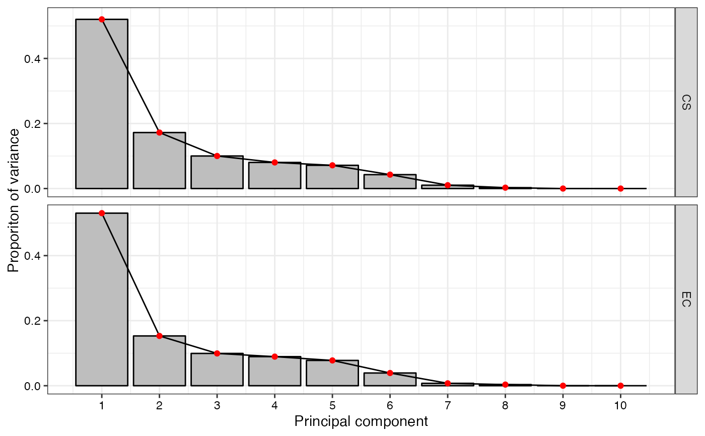
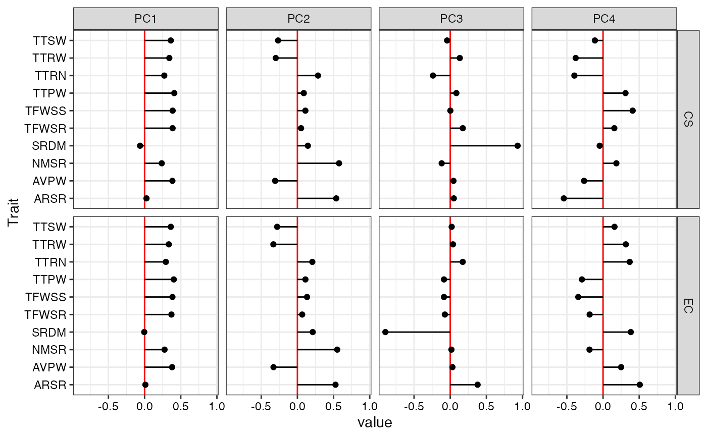
Scree Plot: The scree plot of principal components for EC and CS as a ggplot object.
PC Loadings Plot: A plot of the eigen vector values of principal components for EC and CS as specified by npc.plot as a ggplot2 object.

References

Mardia KV, Kent JT, Bibby JM (1979). Multivariate analysis. Academic Press, London; New York. ISBN 0-12-471250-9 978-0-12-471250-8 0-12-471252-5 978-0-12-471252-2.

Examples


data("cassava_CC")
data("cassava_EC")

ec <- cbind(genotypes = rownames(cassava_EC), cassava_EC)
ec$genotypes <- as.character(ec$genotypes)
rownames(ec) <- NULL

core <- rownames(cassava_CC)

quant <- c("NMSR", "TTRN", "TFWSR", "TTRW", "TFWSS", "TTSW", "TTPW", "AVPW",
           "ARSR", "SRDM")
qual <- c("CUAL", "LNGS", "PTLC", "DSTA", "LFRT", "LBTEF", "CBTR", "NMLB",
          "ANGB", "CUAL9M", "LVC9M", "TNPR9M", "PL9M", "STRP", "STRC",
          "PSTR")

ec[, qual] <- lapply(ec[, qual],
                     function(x) factor(as.factor(x)))

pca.evaluate.core(data = ec, names = "genotypes",
                  quantitative = quant, selected = core,
                  center = TRUE, scale = TRUE, npc.plot = 4)
#> $`EC PC Importance`
#>                             PC1      PC2      PC3       PC4       PC5       PC6
#> Standard deviation     2.303455 1.237223 0.996322 0.9455592 0.8817511 0.6251589
#> Proportion of Variance 0.530590 0.153070 0.099270 0.0894100 0.0777500 0.0390800
#> Cumulative Proportion  0.530590 0.683660 0.782930 0.8723400 0.9500900 0.9891700
#>                             PC7       PC8          PC9        PC10
#> Standard deviation     0.271212 0.1864651 1.549134e-15 1.20846e-15
#> Proportion of Variance 0.007360 0.0034800 0.000000e+00 0.00000e+00
#> Cumulative Proportion  0.996520 1.0000000 1.000000e+00 1.00000e+00
#> 
#> $`EC PC Loadings`
#>                PC1         PC2         PC3        PC4          PC5         PC6
#> NMSR   0.276022186  0.55062492  0.01668655 -0.1871023  0.248244608 -0.21686806
#> TTRN   0.293942565  0.20622412  0.17262243  0.3680853  0.581178024 -0.33878178
#> TFWSR  0.371192088  0.06599302 -0.07379106 -0.1852754 -0.463167012 -0.33058227
#> TTRW   0.334894681 -0.33211659  0.03783194  0.3153475 -0.297171591 -0.40373685
#> TFWSS  0.385024604  0.13341651 -0.08631304 -0.3426523  0.050559491  0.39246657
#> TTSW   0.362255093 -0.27969168  0.02022637  0.1585548  0.250560331  0.51748203
#> TTPW   0.403699747  0.11088360 -0.08613665 -0.2920918 -0.184053823  0.08318831
#> AVPW   0.380627616 -0.33011132  0.03067827  0.2497406  0.002748448  0.10913947
#> ARSR   0.011265368  0.52673026  0.37858111  0.5081543 -0.444763915  0.34913640
#> SRDM  -0.004586239  0.21186429 -0.89638345  0.3837654 -0.027148446  0.05797814
#>               PC7          PC8           PC9          PC10
#> NMSR  -0.66616815  0.181386616  2.716790e-16  2.045788e-15
#> TTRN   0.49417918 -0.095026370 -1.567310e-15 -1.169297e-15
#> TFWSR  0.32960316  0.499641762 -2.002707e-01  3.096651e-01
#> TTRW  -0.31608453 -0.416500300  3.273437e-01  2.117040e-01
#> TFWSS  0.10285083 -0.558642359 -2.603566e-01  4.025719e-01
#> TTSW  -0.07640644  0.454657280  3.955273e-01  2.558006e-01
#> TTPW   0.21455970 -0.104941479  4.324565e-01 -6.686784e-01
#> AVPW  -0.20120313  0.065453705 -6.644485e-01 -4.297208e-01
#> ARSR   0.01979215 -0.027945977 -5.836779e-18  7.484100e-17
#> SRDM   0.01152032 -0.009060183 -7.744396e-17 -8.136954e-17
#> 
#> $`CS PC Importance`
#>                             PC1      PC2      PC3       PC4       PC5       PC6
#> Standard deviation     2.280951 1.312257 1.000457 0.8959377 0.8451336 0.6538375
#> Proportion of Variance 0.520270 0.172200 0.100090 0.0802700 0.0714300 0.0427500
#> Cumulative Proportion  0.520270 0.692480 0.792570 0.8728400 0.9442600 0.9870100
#>                              PC7       PC8          PC9         PC10
#> Standard deviation     0.3207286 0.1643265 8.218513e-16 3.899579e-16
#> Proportion of Variance 0.0102900 0.0027000 0.000000e+00 0.000000e+00
#> Cumulative Proportion  0.9973000 1.0000000 1.000000e+00 1.000000e+00
#> 
#> $`CS PC Loadings`
#>               PC1         PC2          PC3         PC4         PC5          PC6
#> NMSR   0.23686459  0.57588211 -0.118000407  0.18406534  0.22404134 -0.154356246
#> TTRN   0.27243380  0.28489364 -0.238654425 -0.39636509  0.59296937 -0.185643439
#> TFWSR  0.38732336  0.05088131  0.173676592  0.15588284 -0.33283776 -0.410239780
#> TTRW   0.34195710 -0.29955595  0.132403764 -0.37824392 -0.14609160 -0.425032356
#> TFWSS  0.38798499  0.11032791  0.002061297  0.40943370 -0.02293943  0.339541418
#> TTSW   0.36275510 -0.26716740 -0.043442847 -0.11254725  0.18634678  0.589974192
#> TTPW   0.41017366  0.08800885  0.085090829  0.31069206 -0.17398680 -0.002991297
#> AVPW   0.38441017 -0.30812430  0.044838607 -0.26192922  0.02880417  0.110848682
#> ARSR   0.02642625  0.53641424  0.049592980 -0.54225171 -0.54787309  0.334180984
#> SRDM  -0.06233279  0.14455341  0.931570561 -0.04658879  0.31551819  0.073690249
#>               PC7          PC8           PC9          PC10
#> NMSR   0.69455927 -0.089542525 -5.321232e-16  1.466265e-16
#> TTRN  -0.49373454  0.026538022  5.590506e-16 -3.306053e-16
#> TFWSR -0.24125034 -0.553541017  8.413770e-03  3.862264e-01
#> TTRW   0.26321979  0.434887362 -4.150225e-01  9.041080e-03
#> TFWSS -0.17717813  0.557775840  1.001223e-02  4.596024e-01
#> TTSW   0.13648832 -0.424831173 -4.477452e-01  9.753929e-03
#> TTPW  -0.21841109  0.053240284 -1.741566e-02 -7.994501e-01
#> AVPW   0.21517212 -0.012287406  7.917109e-01 -1.724707e-02
#> ARSR  -0.04644065  0.032656495 -9.717546e-17 -1.548356e-16
#> SRDM  -0.01212024  0.009789162  5.912017e-17  1.088709e-16
#> 
#> $`Scree Plot`

#> 
#> $`PC Loadings Plot`

#>

Arguments

Value

References

See also

Examples