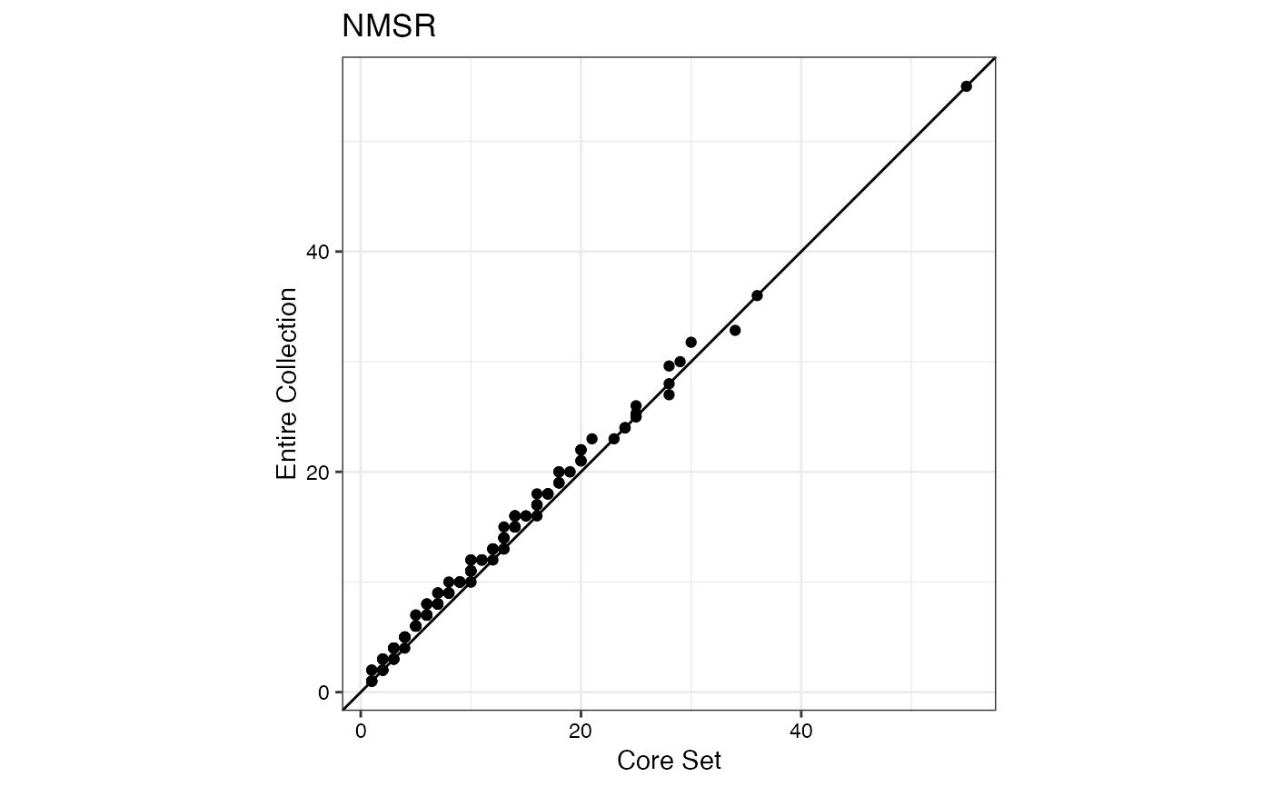
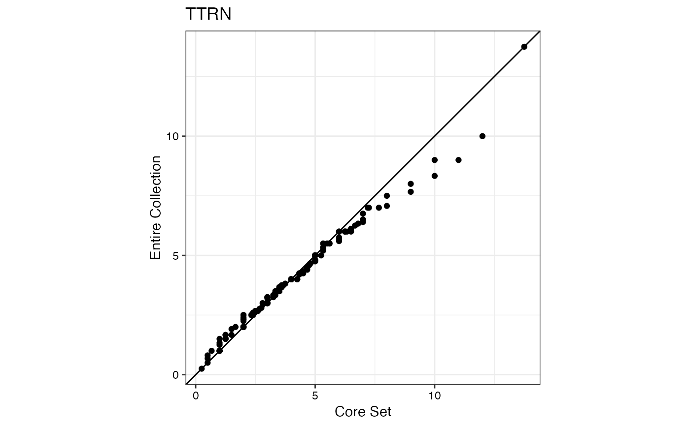
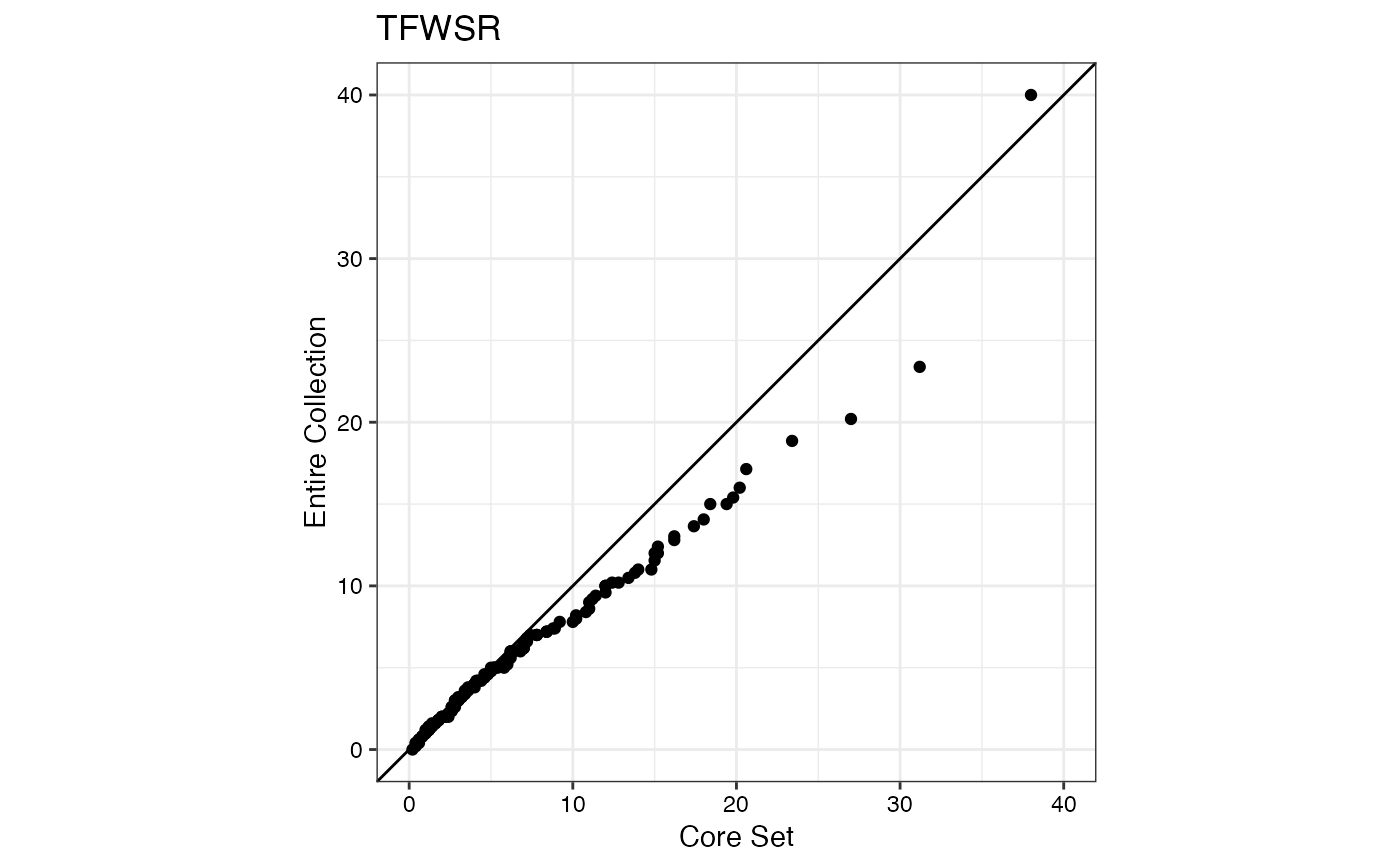
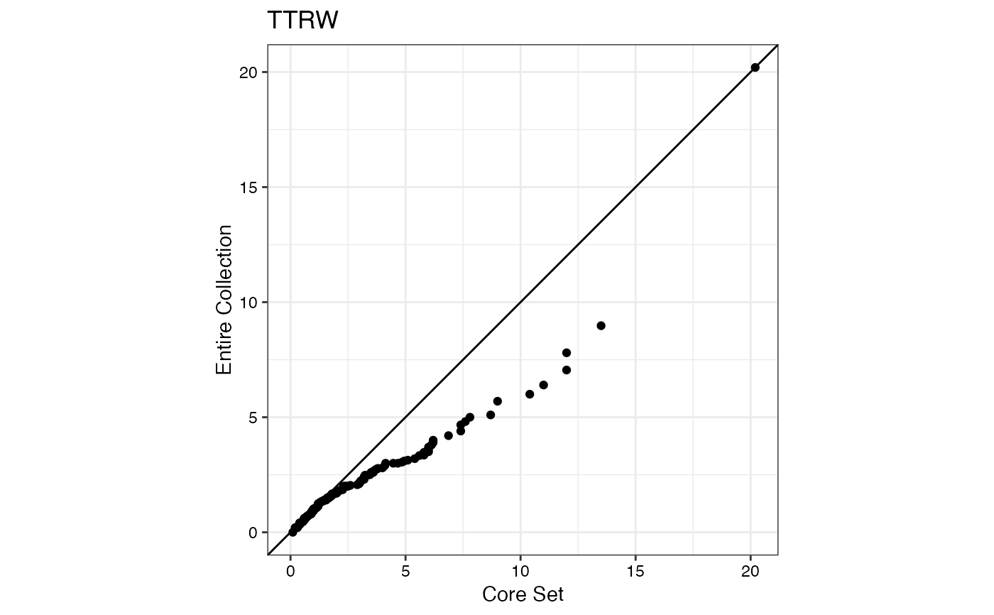
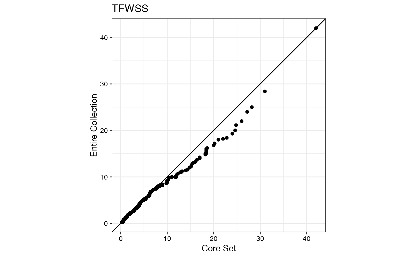
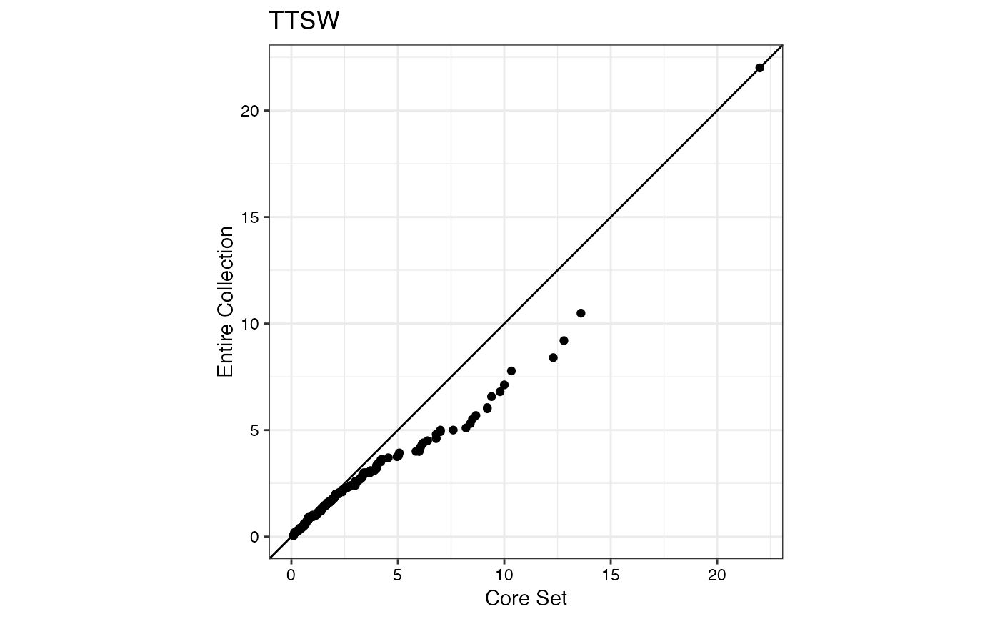
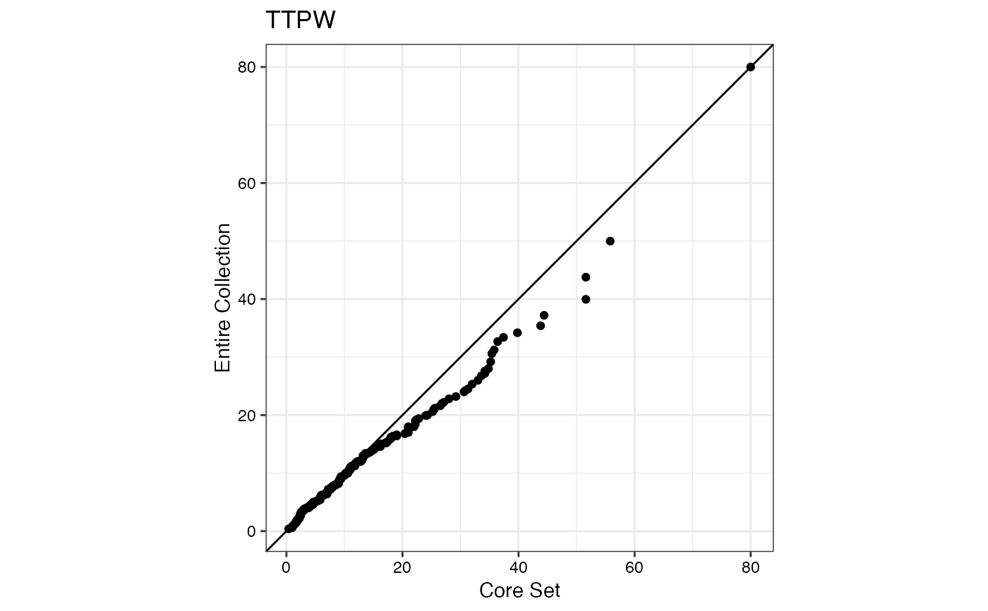
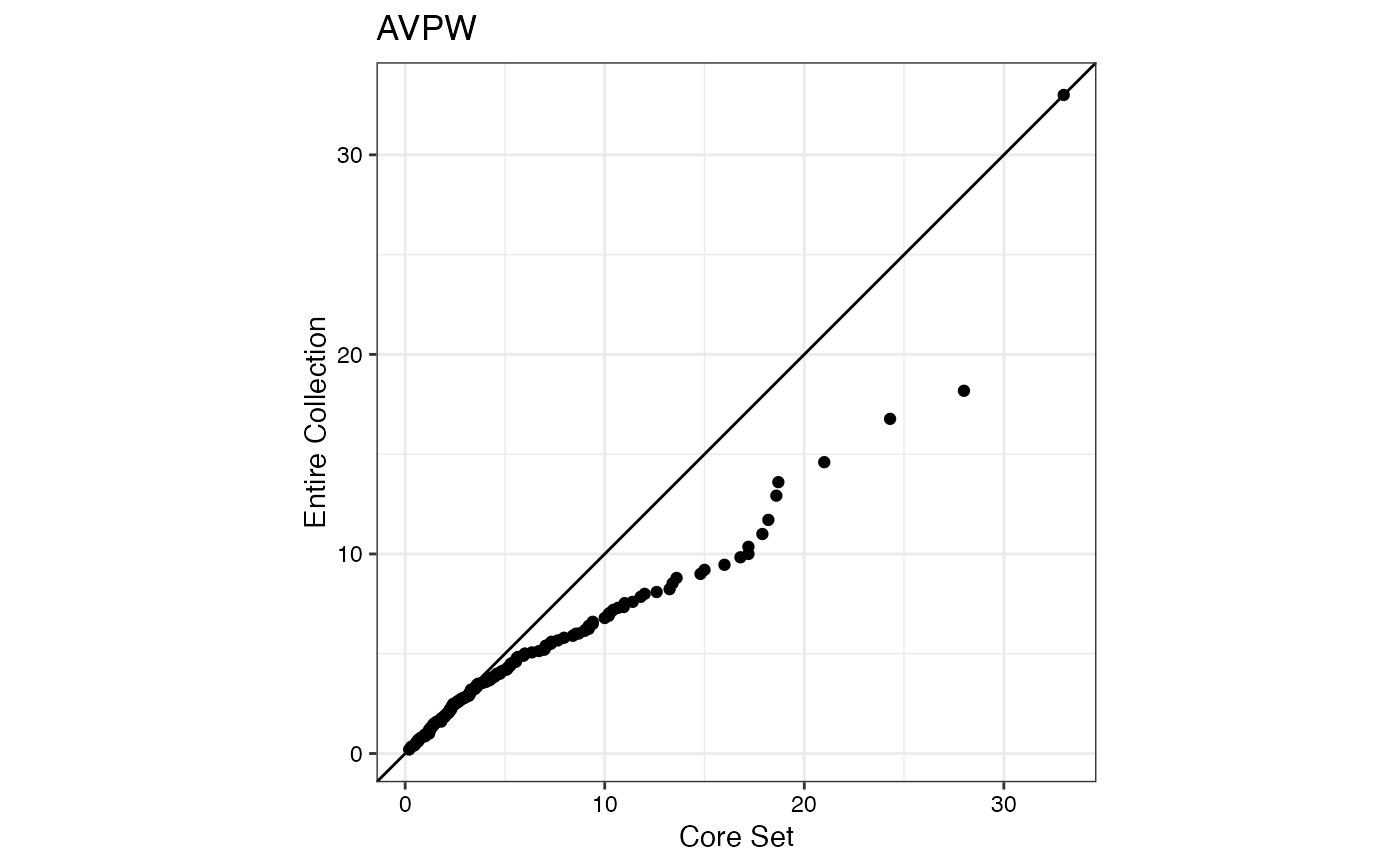
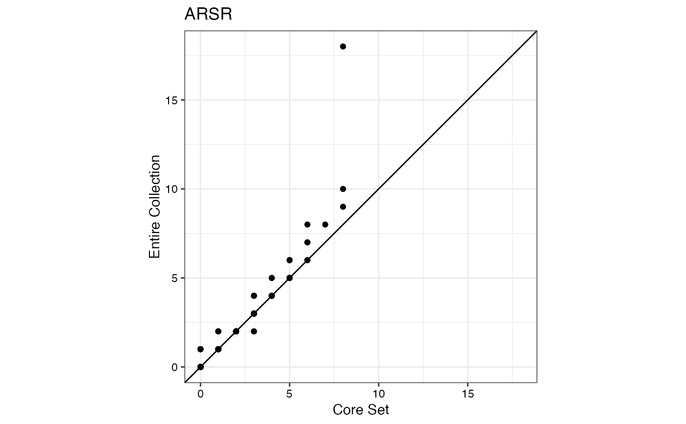
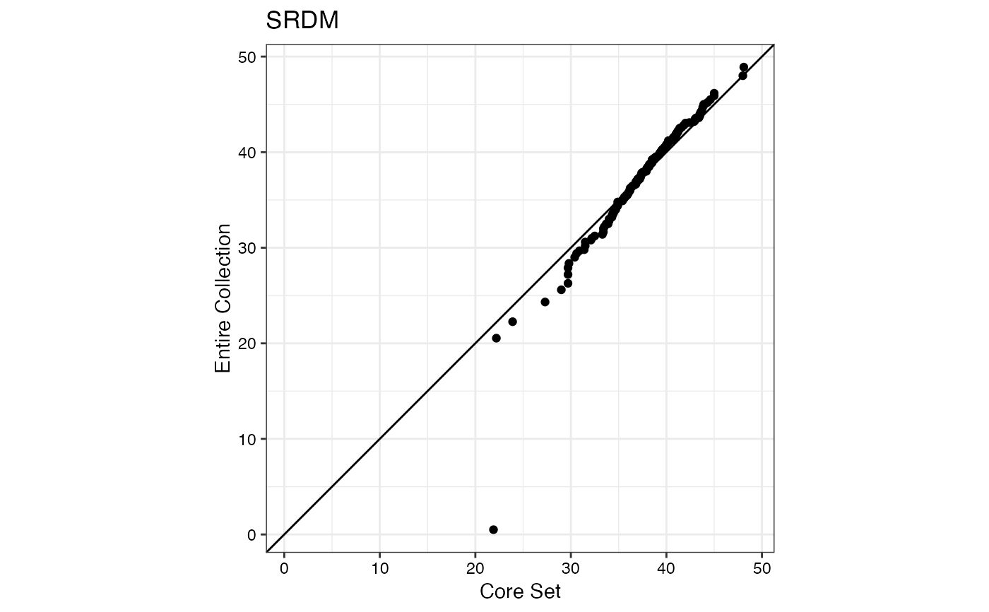
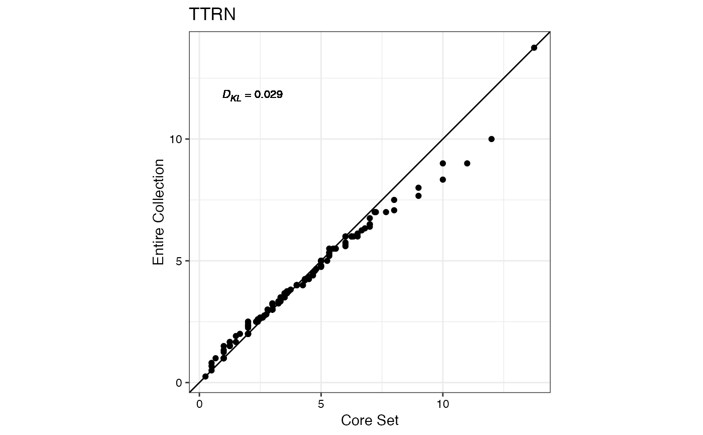
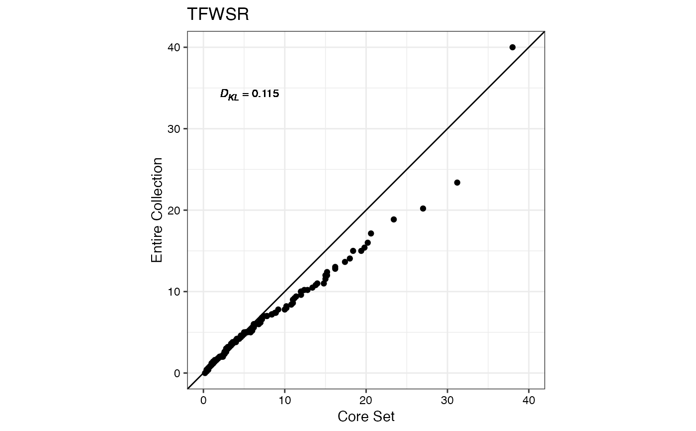
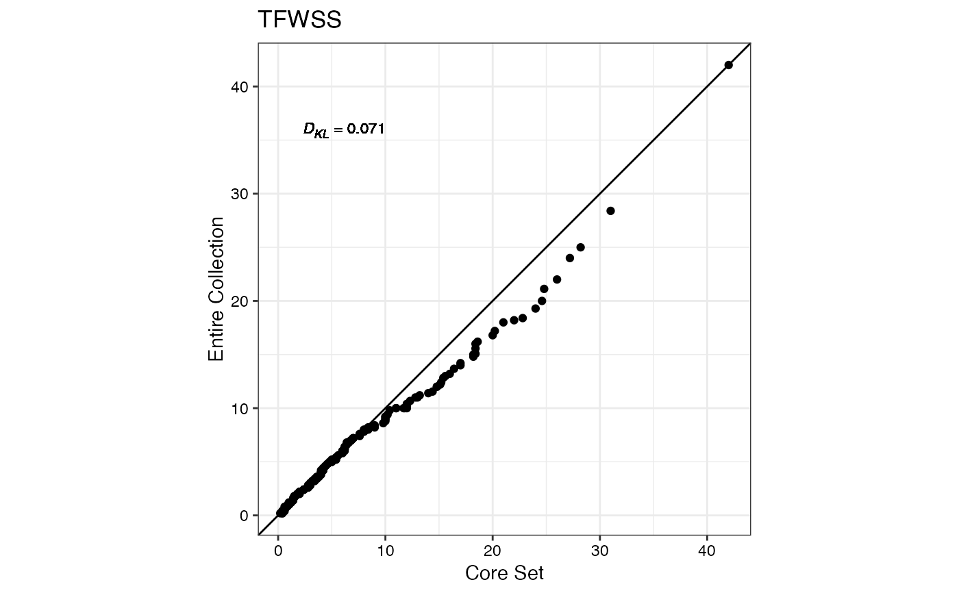
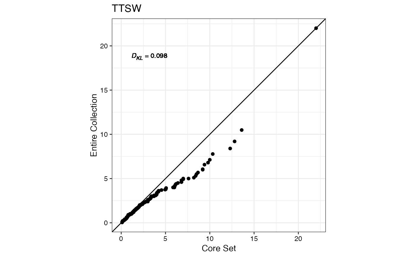
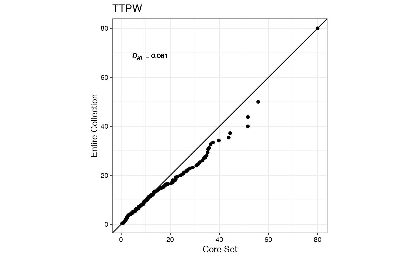
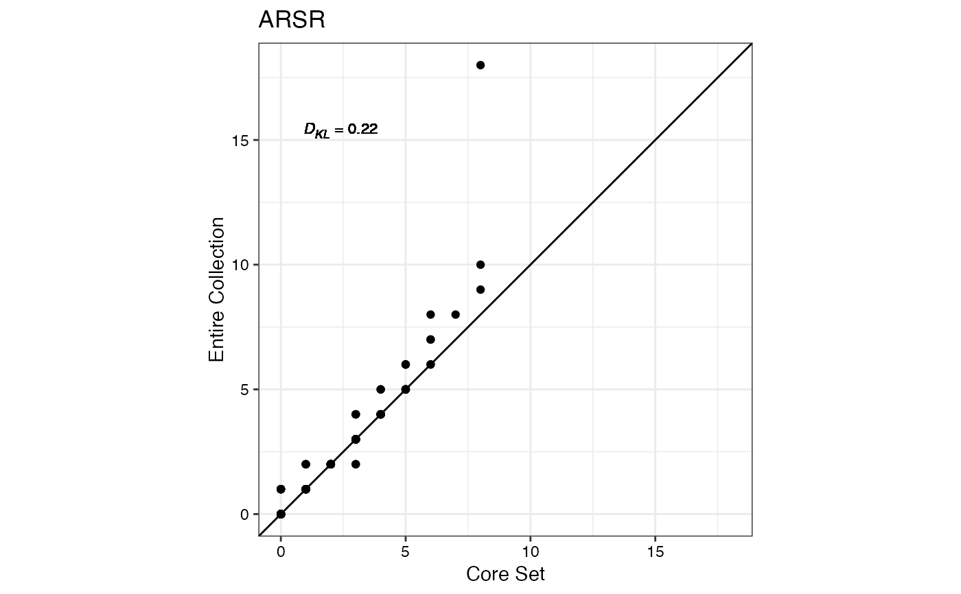
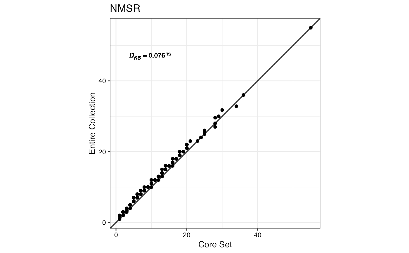
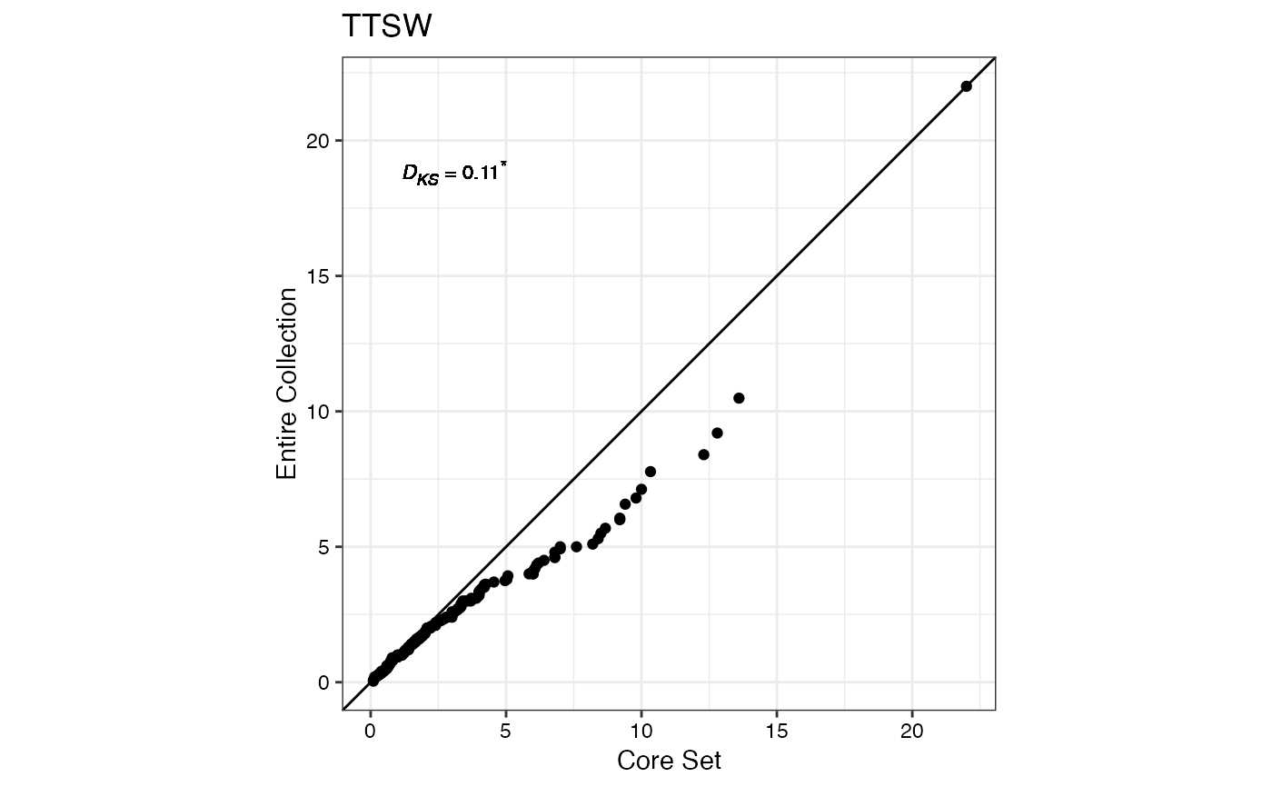
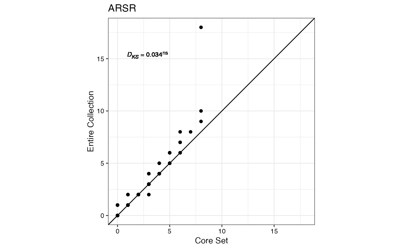
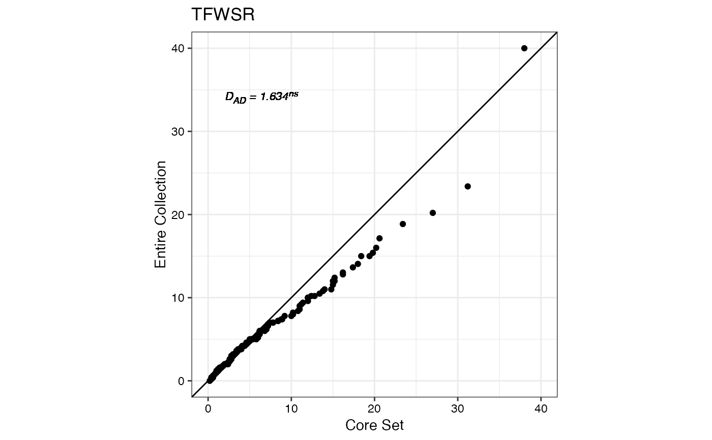
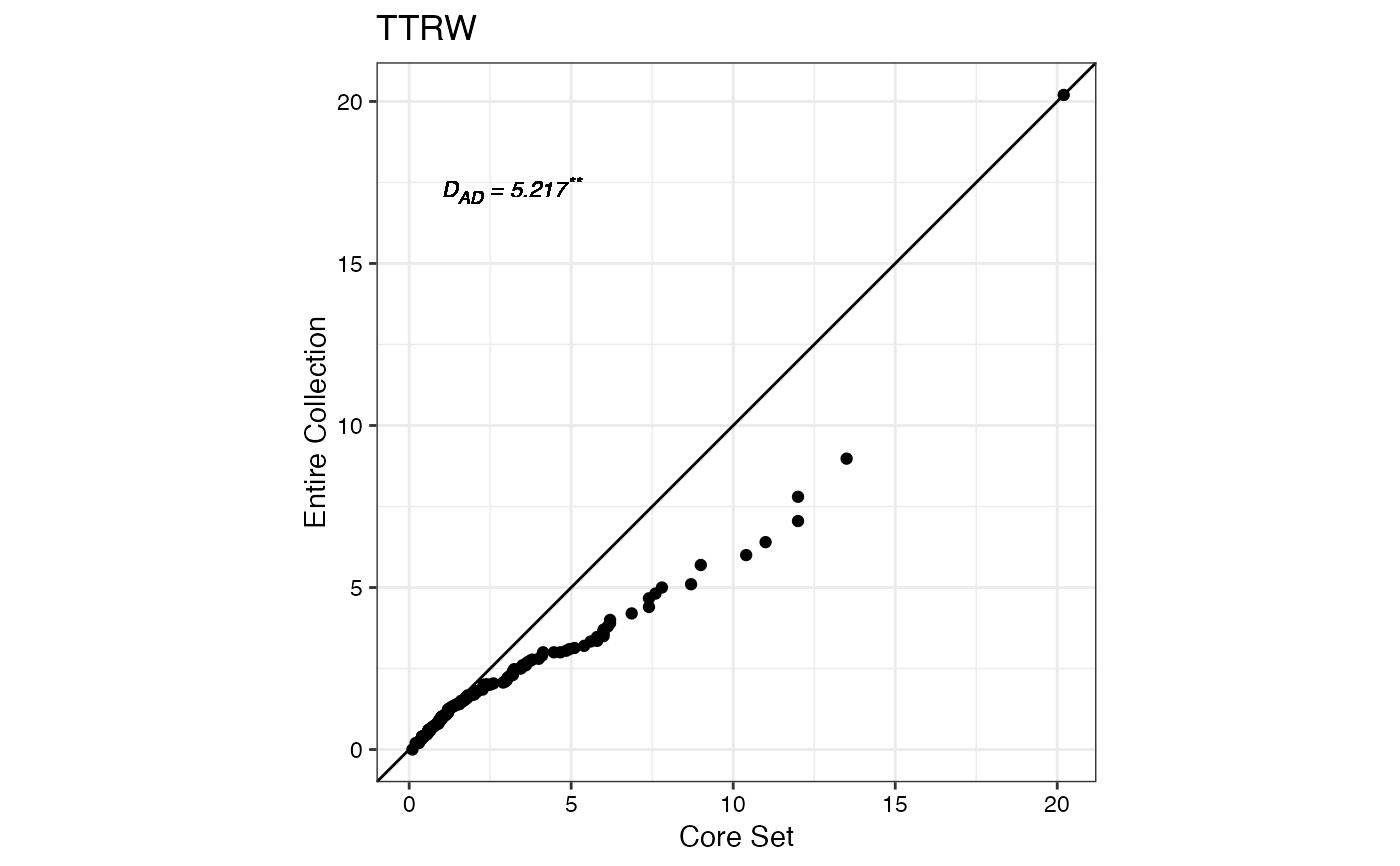
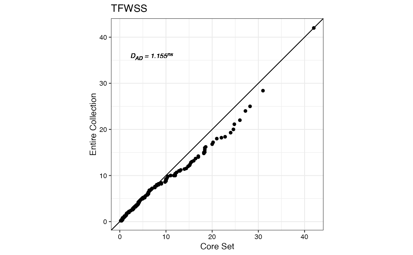
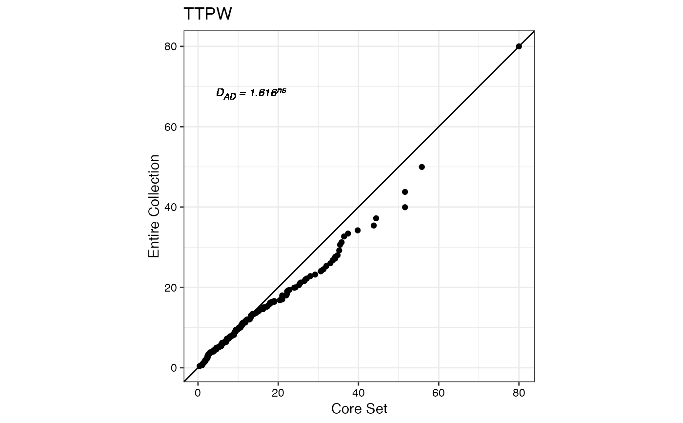
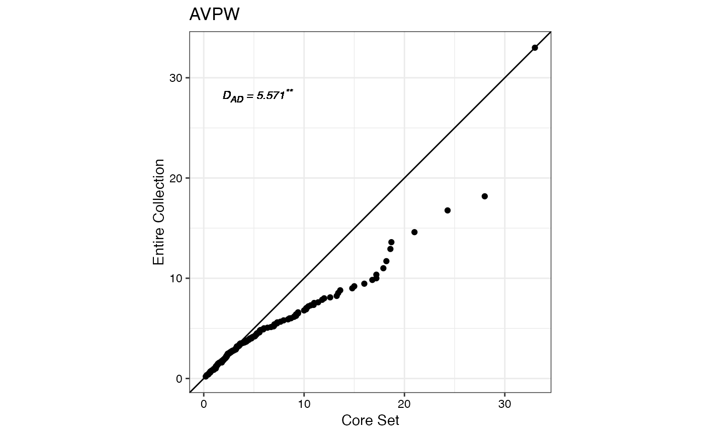
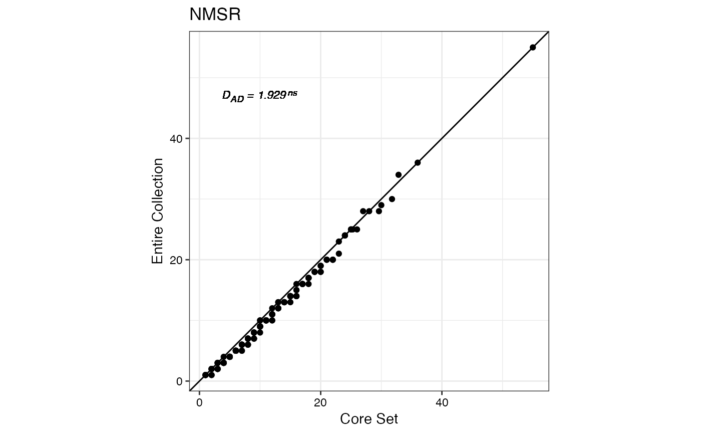
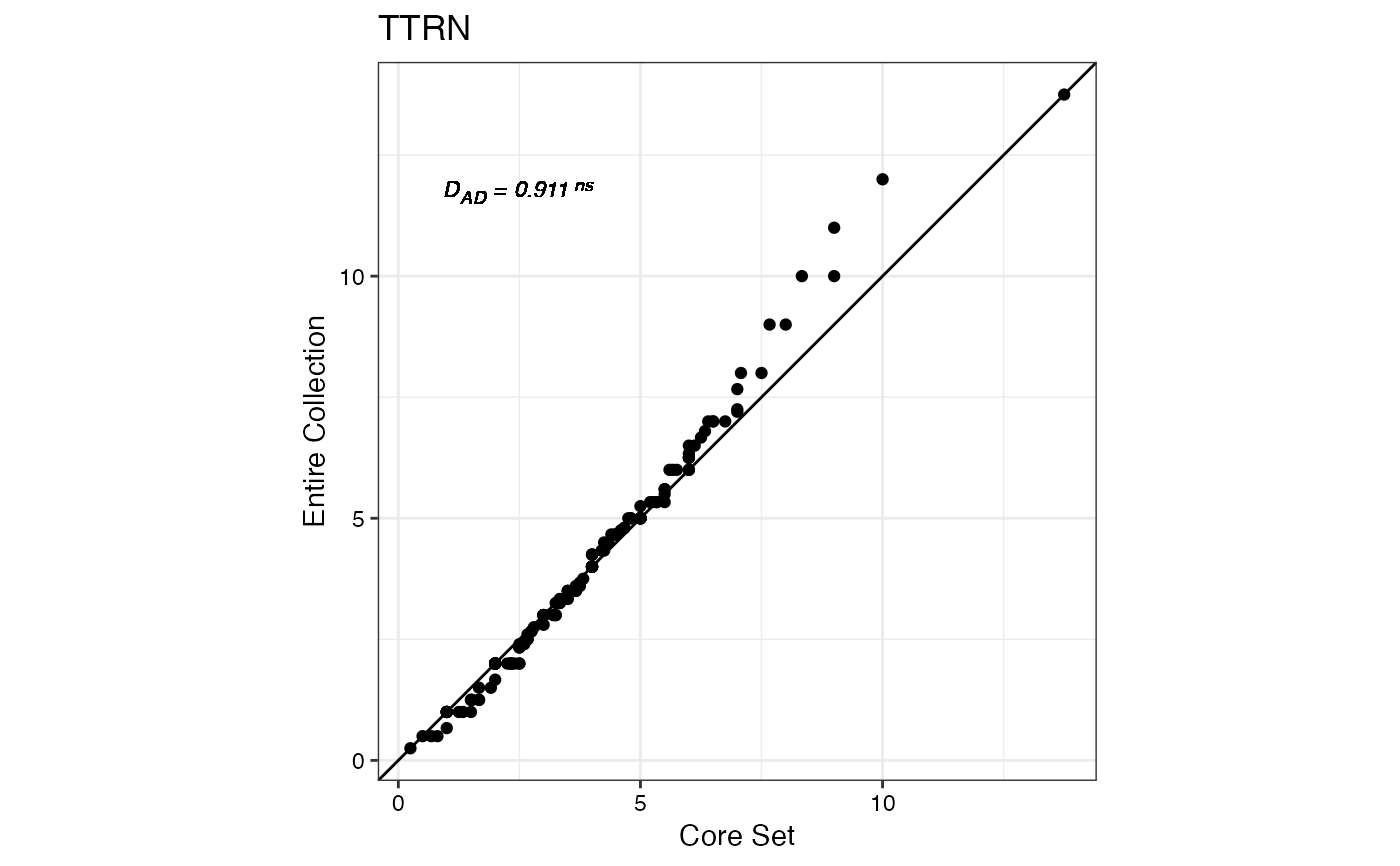
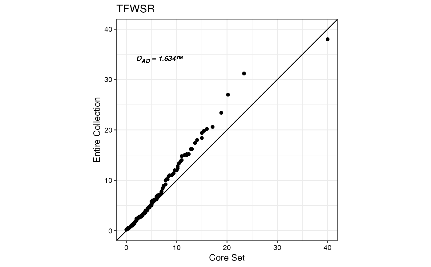
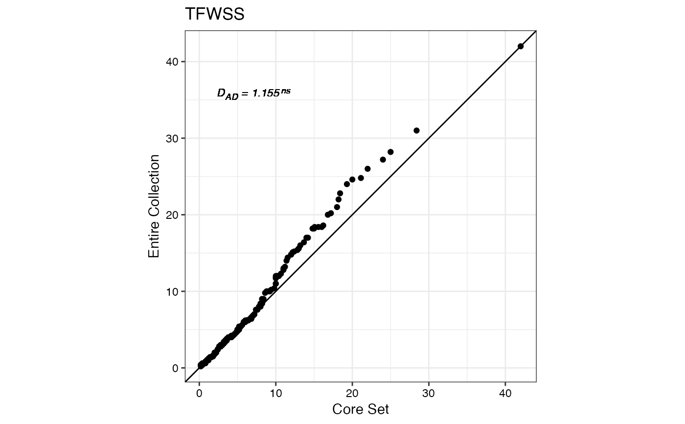
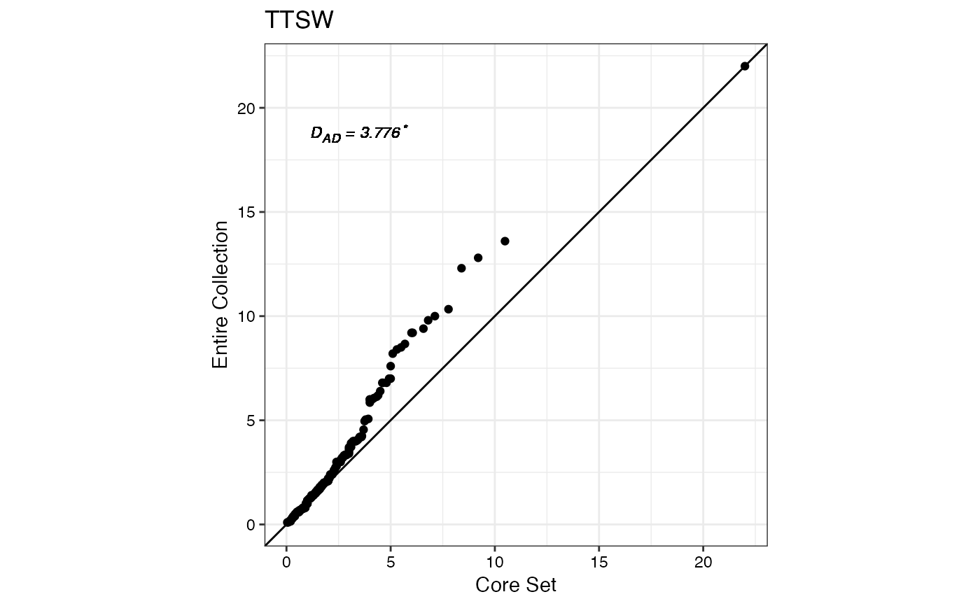
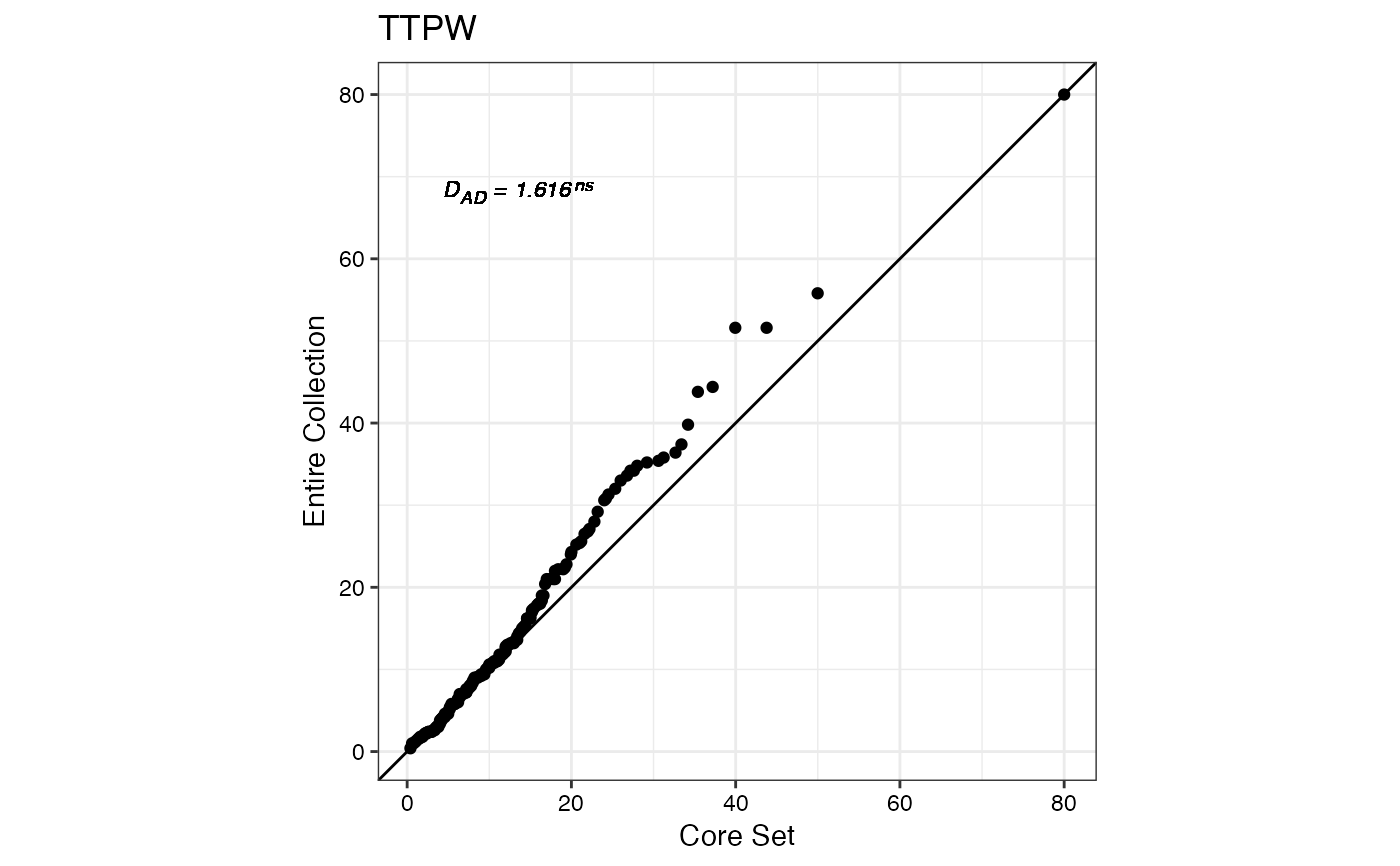
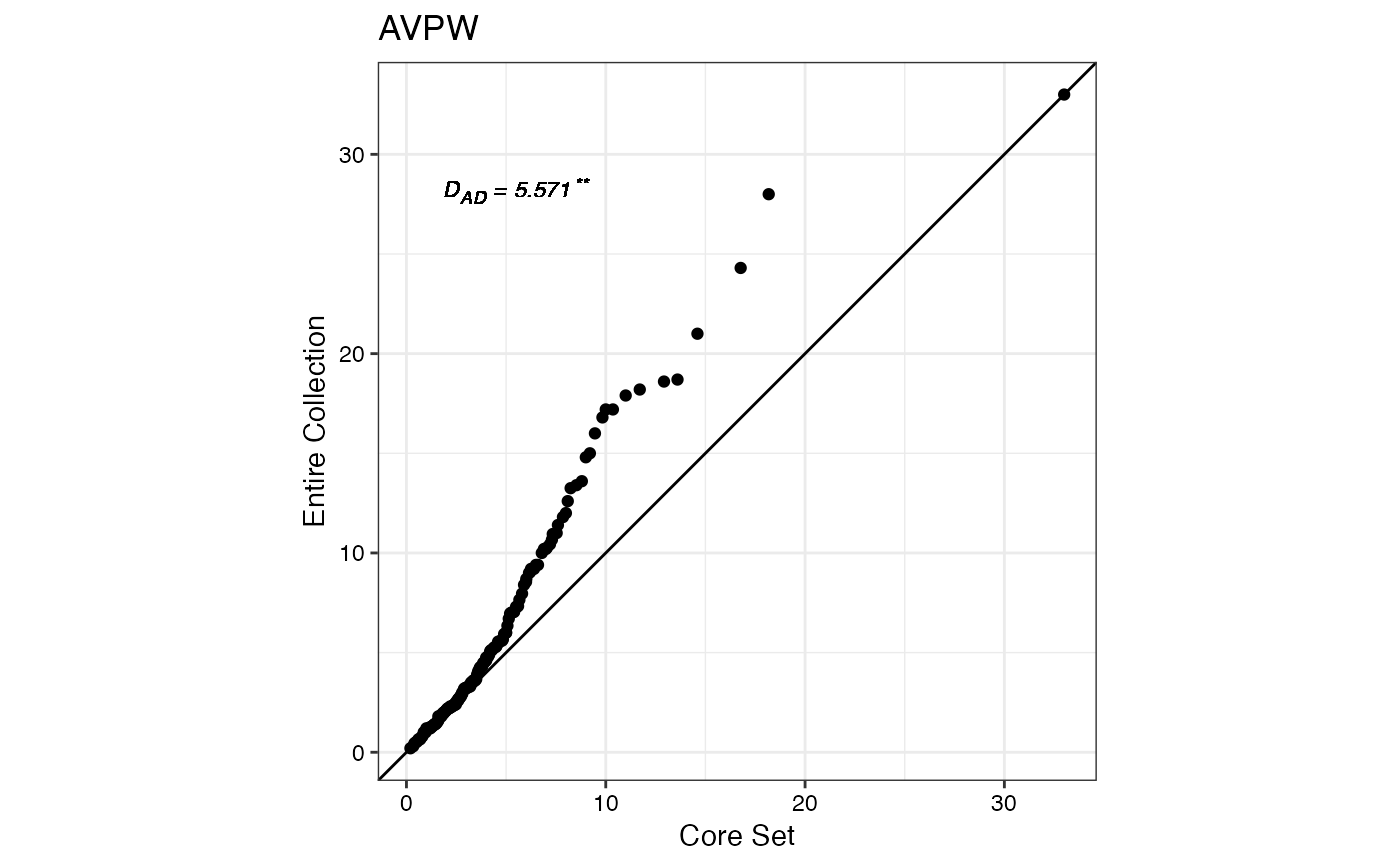
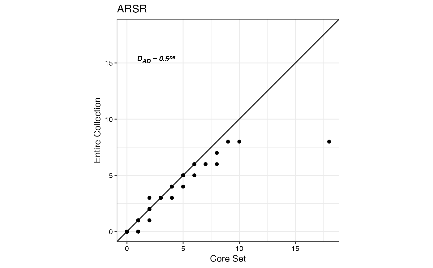
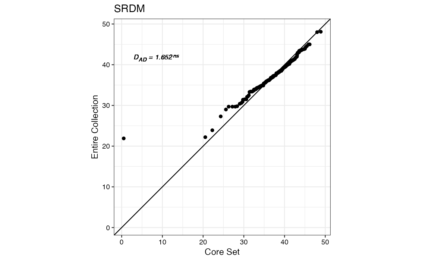
Plot Quantile-Quantile (QQ) plots (Wilk and Gnanadesikan 1968) to graphically compare the probability distributions of quantitative traits between entire collection (EC) and core set (CS).
Usage
qq.evaluate.core(
  data,
  names,
  quantitative,
  selected,
  annotate = c("none", "kl", "ks", "ad"),
  show.count = FALSE
)
Arguments
- data
The data as a data frame object. The data frame should possess one row per individual and columns with the individual names and multiple trait/character data.
- names
Name of column with the individual names as a character string.
- quantitative
Name of columns with the quantitative traits as a character vector.
- selected
Character vector with the names of individuals selected in core collection and present in the
namescolumn.- annotate
Adds the divergence/distance value between probability distributions of CS and EC as an annotation to the QQ plot. Either
"none"(no annotation (Default)) or"kl"(Kullback-Leibler divergence) or"ks"(Kolmogorov-Smirnov distance) or"ad"(Anderson-Darling distance).- show.count
logical. If
TRUE, the accession count excluding missing values will also be displayed. Default isFALSE.
Value
A list with the ggplot objects of QQ plots of CS vs EC for
each trait specified as quantitative.
References
Wilk MB, Gnanadesikan R (1968). “Probability plotting methods for the analysis for the analysis of data.” Biometrika, 55(1), 1–17.
Examples
data("cassava_CC")
data("cassava_EC")
ec <- cbind(genotypes = rownames(cassava_EC), cassava_EC)
ec$genotypes <- as.character(ec$genotypes)
rownames(ec) <- NULL
core <- rownames(cassava_CC)
quant <- c("NMSR", "TTRN", "TFWSR", "TTRW", "TFWSS", "TTSW", "TTPW", "AVPW",
"ARSR", "SRDM")
qual <- c("CUAL", "LNGS", "PTLC", "DSTA", "LFRT", "LBTEF", "CBTR", "NMLB",
"ANGB", "CUAL9M", "LVC9M", "TNPR9M", "PL9M", "STRP", "STRC",
"PSTR")
ec[, qual] <- lapply(ec[, qual],
function(x) factor(as.factor(x)))
# \donttest{
qq.evaluate.core(data = ec, names = "genotypes",
quantitative = quant, selected = core)
#> $NMSR
 #>
#> $TTRN
#>
#> $TTRN
 #>
#> $TFWSR
#>
#> $TFWSR
 #>
#> $TTRW
#>
#> $TTRW
 #>
#> $TFWSS
#>
#> $TFWSS
 #>
#> $TTSW
#>
#> $TTSW
 #>
#> $TTPW
#>
#> $TTPW
 #>
#> $AVPW
#>
#> $AVPW
 #>
#> $ARSR
#>
#> $ARSR
 #>
#> $SRDM
#>
#> $SRDM
 #>
qq.evaluate.core(data = ec, names = "genotypes",
quantitative = quant, selected = core, show.count = TRUE)
#> $NMSR
#>
qq.evaluate.core(data = ec, names = "genotypes",
quantitative = quant, selected = core, show.count = TRUE)
#> $NMSR
 #>
#> $TTRN
#>
#> $TTRN
 #>
#> $TFWSR
#>
#> $TFWSR
 #>
#> $TTRW
#>
#> $TTRW
 #>
#> $TFWSS
#>
#> $TFWSS
 #>
#> $TTSW
#>
#> $TTSW
 #>
#> $TTPW
#>
#> $TTPW
 #>
#> $AVPW
#>
#> $AVPW
 #>
#> $ARSR
#>
#> $ARSR
 #>
#> $SRDM
#>
#> $SRDM
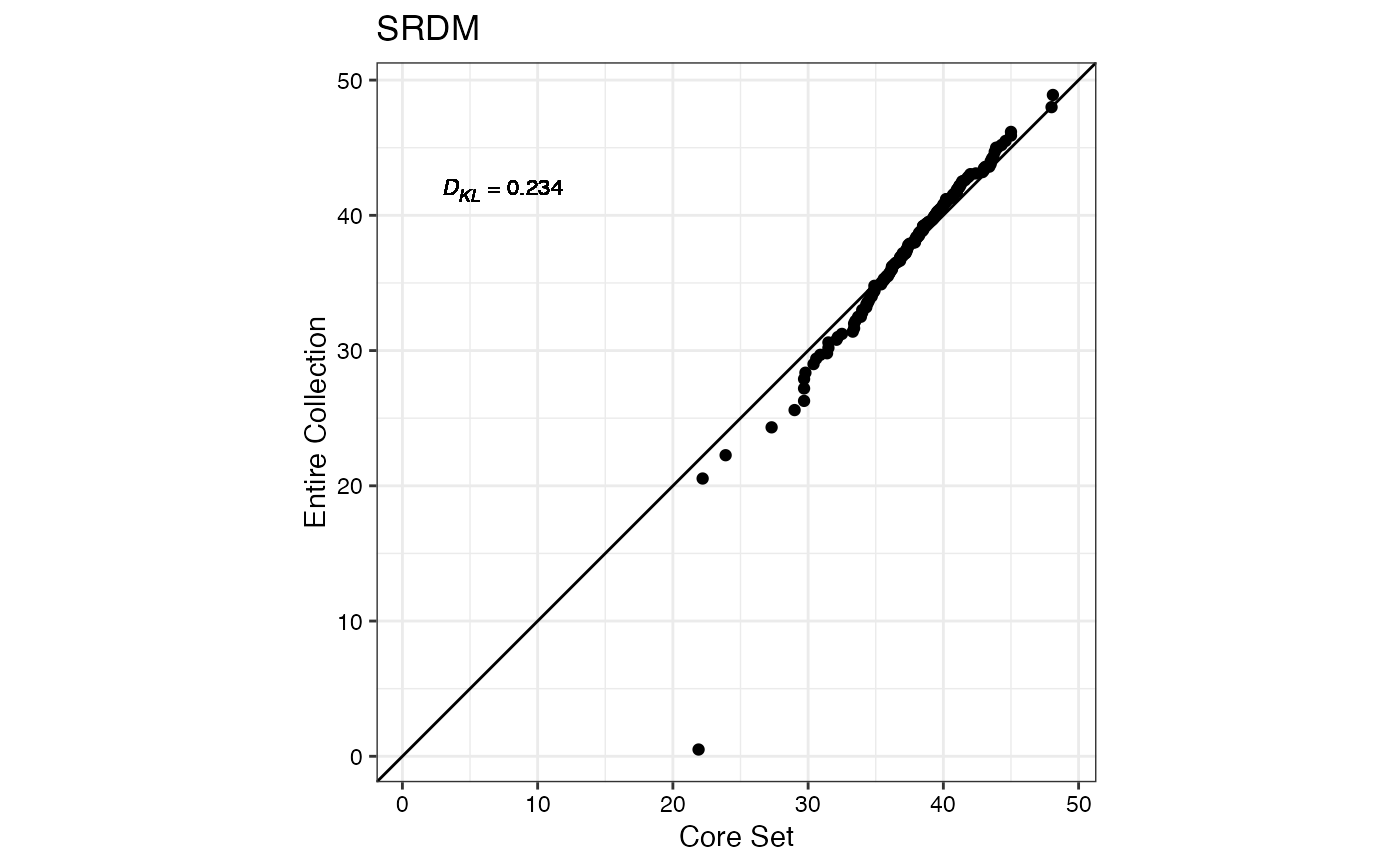 #>
qq.evaluate.core(data = ec, names = "genotypes",
quantitative = quant, selected = core, annotate = "kl")
#> $NMSR
#>
qq.evaluate.core(data = ec, names = "genotypes",
quantitative = quant, selected = core, annotate = "kl")
#> $NMSR
 #>
#> $TTRN
#>
#> $TTRN
 #>
#> $TFWSR
#>
#> $TFWSR
 #>
#> $TTRW
#>
#> $TTRW
 #>
#> $TFWSS
#>
#> $TFWSS
 #>
#> $TTSW
#>
#> $TTSW
 #>
#> $TTPW
#>
#> $TTPW
 #>
#> $AVPW
#>
#> $AVPW
 #>
#> $ARSR
#>
#> $ARSR
 #>
#> $SRDM
#>
#> $SRDM
 #>
qq.evaluate.core(data = ec, names = "genotypes",
quantitative = quant, selected = core, annotate = "ks")
#> Warning: p-value will be approximate in the presence of ties
#> Warning: p-value will be approximate in the presence of ties
#> Warning: p-value will be approximate in the presence of ties
#> Warning: p-value will be approximate in the presence of ties
#> Warning: p-value will be approximate in the presence of ties
#> Warning: p-value will be approximate in the presence of ties
#> Warning: p-value will be approximate in the presence of ties
#> Warning: p-value will be approximate in the presence of ties
#> Warning: p-value will be approximate in the presence of ties
#> Warning: p-value will be approximate in the presence of ties
#> $NMSR
#>
qq.evaluate.core(data = ec, names = "genotypes",
quantitative = quant, selected = core, annotate = "ks")
#> Warning: p-value will be approximate in the presence of ties
#> Warning: p-value will be approximate in the presence of ties
#> Warning: p-value will be approximate in the presence of ties
#> Warning: p-value will be approximate in the presence of ties
#> Warning: p-value will be approximate in the presence of ties
#> Warning: p-value will be approximate in the presence of ties
#> Warning: p-value will be approximate in the presence of ties
#> Warning: p-value will be approximate in the presence of ties
#> Warning: p-value will be approximate in the presence of ties
#> Warning: p-value will be approximate in the presence of ties
#> $NMSR
 #>
#> $TTRN
#>
#> $TTRN
 #>
#> $TFWSR
#>
#> $TFWSR
 #>
#> $TTRW
#>
#> $TTRW
 #>
#> $TFWSS
#>
#> $TFWSS
 #>
#> $TTSW
#>
#> $TTSW
 #>
#> $TTPW
#>
#> $TTPW
 #>
#> $AVPW
#>
#> $AVPW
 #>
#> $ARSR
#>
#> $ARSR
 #>
#> $SRDM
#>
#> $SRDM
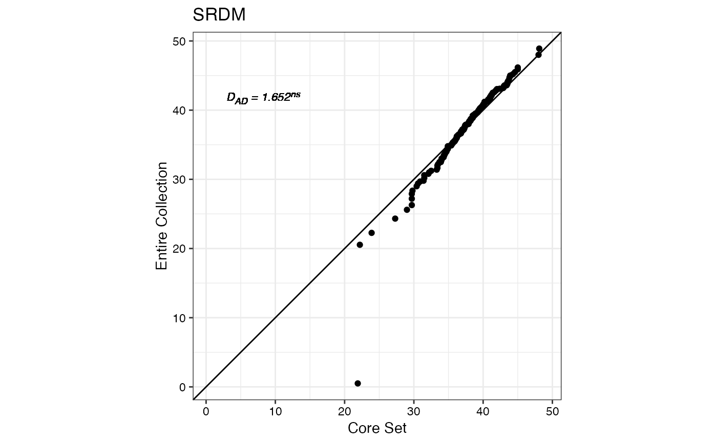 #>
qq.evaluate.core(data = ec, names = "genotypes",
quantitative = quant, selected = core, annotate = "ad")
#> $NMSR
#>
qq.evaluate.core(data = ec, names = "genotypes",
quantitative = quant, selected = core, annotate = "ad")
#> $NMSR
 #>
#> $TTRN
#>
#> $TTRN
 #>
#> $TFWSR
#>
#> $TFWSR
 #>
#> $TTRW
#>
#> $TTRW
 #>
#> $TFWSS
#>
#> $TFWSS
 #>
#> $TTSW
#>
#> $TTSW
 #>
#> $TTPW
#>
#> $TTPW
 #>
#> $AVPW
#>
#> $AVPW
 #>
#> $ARSR
#>
#> $ARSR
 #>
#> $SRDM
#>
#> $SRDM
 #>
# }
#>
# }