Plot Frequency Distribution from augmentedRCBD Output
Source: R/freqdist.augmentedRCBD.R
freqdist.augmentedRCBD.Rdfreqdist.augmentedRCBD plots frequency distribution from an object of
class augmentedRCBD along with the corresponding normal curve and
check means with standard errors (if specified by argument
highlight.check).
Arguments
- aug
An object of class
augmentedRCBD.- xlab
The text for x axis label as a character string.
- highlight.check
If
TRUE, the check means and standard errors are also plotted. Default isTRUE.- check.col
The colour(s) to be used to highlight check values in the plot as a character vector. Must be valid colour values in R (named colours, hexadecimal representation, index of colours [
1:8] in default Rpalette()etc.).
Examples
# Example data
blk <- c(rep(1,7),rep(2,6),rep(3,7))
trt <- c(1, 2, 3, 4, 7, 11, 12, 1, 2, 3, 4, 5, 9, 1, 2, 3, 4, 8, 6, 10)
y1 <- c(92, 79, 87, 81, 96, 89, 82, 79, 81, 81, 91, 79, 78, 83, 77, 78, 78,
70, 75, 74)
y2 <- c(258, 224, 238, 278, 347, 300, 289, 260, 220, 237, 227, 281, 311,
250, 240, 268, 287, 226, 395, 450)
data <- data.frame(blk, trt, y1, y2)
# Convert block and treatment to factors
data$blk <- as.factor(data$blk)
data$trt <- as.factor(data$trt)
# Results for variable y1
out1 <- augmentedRCBD(block = data$blk, treatment = data$trt, y = data$y1,
method.comp = "lsd", alpha = 0.05, group = TRUE,
console = TRUE)
#>
#> Augmented Design Details
#> ========================
#>
#> Number of blocks "3"
#> Number of treatments "12"
#> Number of check treatments "4"
#> Number of test treatments "8"
#> Check treatments "1, 2, 3, 4"
#>
#>
#> ANOVA, Treatment Adjusted
#> =========================
#> Df Sum Sq Mean Sq F value Pr(>F)
#> Block (ignoring Treatments) 2 360.1 180.04 6.675 0.0298 *
#> Treatment (eliminating Blocks) 11 285.1 25.92 0.961 0.5499
#> Treatment: Check 3 52.9 17.64 0.654 0.6092
#> Treatment: Test and Test vs. Check 8 232.2 29.02 1.076 0.4779
#> Residuals 6 161.8 26.97
#> ---
#> Signif. codes: 0 ‘***’ 0.001 ‘**’ 0.01 ‘*’ 0.05 ‘.’ 0.1 ‘ ’ 1
#>
#> ANOVA, Block Adjusted
#> =====================
#> Df Sum Sq Mean Sq F value Pr(>F)
#> Treatment (ignoring Blocks) 11 575.7 52.33 1.940 0.215
#> Treatment: Check 3 52.9 17.64 0.654 0.609
#> Treatment: Test 7 505.9 72.27 2.679 0.125
#> Treatment: Test vs. Check 1 16.9 16.87 0.626 0.459
#> Block (eliminating Treatments) 2 69.5 34.75 1.288 0.342
#> Residuals 6 161.8 26.97
#>
#> Coefficient of Variation
#> ========================
#> 6.372367
#>
#> Overall Adjusted Mean
#> =====================
#> 81.0625
#>
#> Standard Errors
#> ===============
#> Std. Error of Diff. CD (5%)
#> Control Treatment Means 4.240458 10.37603
#> Two Test Treatments (Same Block) 7.344688 17.97180
#> Two Test Treatments (Different Blocks) 8.211611 20.09309
#> A Test Treatment and a Control Treatment 6.704752 16.40594
#>
#> Treatment Means
#> ===============
#> Treatment Block Means SE r Min Max Adjusted Means
#> 1 84.67 3.84 3 79.00 92.00 84.67
#> 10 3 74.00 <NA> 1 74.00 74.00 77.25
#> 11 1 89.00 <NA> 1 89.00 89.00 86.50
#> 12 1 82.00 <NA> 1 82.00 82.00 79.50
#> 2 79.00 1.15 3 77.00 81.00 79.00
#> 3 82.00 2.65 3 78.00 87.00 82.00
#> 4 83.33 3.93 3 78.00 91.00 83.33
#> 5 2 79.00 <NA> 1 79.00 79.00 78.25
#> 6 3 75.00 <NA> 1 75.00 75.00 78.25
#> 7 1 96.00 <NA> 1 96.00 96.00 93.50
#> 8 3 70.00 <NA> 1 70.00 70.00 73.25
#> 9 2 78.00 <NA> 1 78.00 78.00 77.25
#>
#>
#> Comparisons
#> ===========
#>
#> Method : lsd
#>
#> contrast estimate SE df t.ratio p.value sig
#> treatment1 - treatment2 5.67 4.24 6 1.336 0.230
#> treatment1 - treatment3 2.67 4.24 6 0.629 0.553
#> treatment1 - treatment4 1.33 4.24 6 0.314 0.764
#> treatment1 - treatment5 6.42 6.36 6 1.009 0.352
#> treatment1 - treatment6 6.42 6.36 6 1.009 0.352
#> treatment1 - treatment7 -8.83 6.36 6 -1.389 0.214
#> treatment1 - treatment8 11.42 6.36 6 1.795 0.123
#> treatment1 - treatment9 7.42 6.36 6 1.166 0.288
#> treatment1 - treatment10 7.42 6.36 6 1.166 0.288
#> treatment1 - treatment11 -1.83 6.36 6 -0.288 0.783
#> treatment1 - treatment12 5.17 6.36 6 0.812 0.448
#> treatment2 - treatment3 -3.00 4.24 6 -0.707 0.506
#> treatment2 - treatment4 -4.33 4.24 6 -1.022 0.346
#> treatment2 - treatment5 0.75 6.36 6 0.118 0.910
#> treatment2 - treatment6 0.75 6.36 6 0.118 0.910
#> treatment2 - treatment7 -14.50 6.36 6 -2.280 0.063
#> treatment2 - treatment8 5.75 6.36 6 0.904 0.401
#> treatment2 - treatment9 1.75 6.36 6 0.275 0.792
#> treatment2 - treatment10 1.75 6.36 6 0.275 0.792
#> treatment2 - treatment11 -7.50 6.36 6 -1.179 0.283
#> treatment2 - treatment12 -0.50 6.36 6 -0.079 0.940
#> treatment3 - treatment4 -1.33 4.24 6 -0.314 0.764
#> treatment3 - treatment5 3.75 6.36 6 0.590 0.577
#> treatment3 - treatment6 3.75 6.36 6 0.590 0.577
#> treatment3 - treatment7 -11.50 6.36 6 -1.808 0.121
#> treatment3 - treatment8 8.75 6.36 6 1.376 0.218
#> treatment3 - treatment9 4.75 6.36 6 0.747 0.483
#> treatment3 - treatment10 4.75 6.36 6 0.747 0.483
#> treatment3 - treatment11 -4.50 6.36 6 -0.707 0.506
#> treatment3 - treatment12 2.50 6.36 6 0.393 0.708
#> treatment4 - treatment5 5.08 6.36 6 0.799 0.455
#> treatment4 - treatment6 5.08 6.36 6 0.799 0.455
#> treatment4 - treatment7 -10.17 6.36 6 -1.598 0.161
#> treatment4 - treatment8 10.08 6.36 6 1.585 0.164
#> treatment4 - treatment9 6.08 6.36 6 0.956 0.376
#> treatment4 - treatment10 6.08 6.36 6 0.956 0.376
#> treatment4 - treatment11 -3.17 6.36 6 -0.498 0.636
#> treatment4 - treatment12 3.83 6.36 6 0.603 0.569
#> treatment5 - treatment6 0.00 8.21 6 0.000 1.000
#> treatment5 - treatment7 -15.25 8.21 6 -1.857 0.113
#> treatment5 - treatment8 5.00 8.21 6 0.609 0.565
#> treatment5 - treatment9 1.00 7.34 6 0.136 0.896
#> treatment5 - treatment10 1.00 8.21 6 0.122 0.907
#> treatment5 - treatment11 -8.25 8.21 6 -1.005 0.354
#> treatment5 - treatment12 -1.25 8.21 6 -0.152 0.884
#> treatment6 - treatment7 -15.25 8.21 6 -1.857 0.113
#> treatment6 - treatment8 5.00 7.34 6 0.681 0.521
#> treatment6 - treatment9 1.00 8.21 6 0.122 0.907
#> treatment6 - treatment10 1.00 7.34 6 0.136 0.896
#> treatment6 - treatment11 -8.25 8.21 6 -1.005 0.354
#> treatment6 - treatment12 -1.25 8.21 6 -0.152 0.884
#> treatment7 - treatment8 20.25 8.21 6 2.466 0.049 *
#> treatment7 - treatment9 16.25 8.21 6 1.979 0.095
#> treatment7 - treatment10 16.25 8.21 6 1.979 0.095
#> treatment7 - treatment11 7.00 7.34 6 0.953 0.377
#> treatment7 - treatment12 14.00 7.34 6 1.906 0.105
#> treatment8 - treatment9 -4.00 8.21 6 -0.487 0.643
#> treatment8 - treatment10 -4.00 7.34 6 -0.545 0.606
#> treatment8 - treatment11 -13.25 8.21 6 -1.614 0.158
#> treatment8 - treatment12 -6.25 8.21 6 -0.761 0.475
#> treatment9 - treatment10 -0.00 8.21 6 -0.000 1.000
#> treatment9 - treatment11 -9.25 8.21 6 -1.126 0.303
#> treatment9 - treatment12 -2.25 8.21 6 -0.274 0.793
#> treatment10 - treatment11 -9.25 8.21 6 -1.126 0.303
#> treatment10 - treatment12 -2.25 8.21 6 -0.274 0.793
#> treatment11 - treatment12 7.00 7.34 6 0.953 0.377
#>
#> Treatment Groups
#> ================
#>
#> Method : lsd
#>
#> Treatment Adjusted Means SE df lower.CL upper.CL Group
#> 8 73.25 5.61 6 59.52 86.98 1
#> 9 77.25 5.61 6 63.52 90.98 12
#> 10 77.25 5.61 6 63.52 90.98 12
#> 5 78.25 5.61 6 64.52 91.98 12
#> 6 78.25 5.61 6 64.52 91.98 12
#> 2 79.00 3.00 6 71.66 86.34 12
#> 12 79.50 5.61 6 65.77 93.23 12
#> 3 82.00 3.00 6 74.66 89.34 12
#> 4 83.33 3.00 6 76.00 90.67 12
#> 1 84.67 3.00 6 77.33 92.00 12
#> 11 86.50 5.61 6 72.77 100.23 12
#> 7 93.50 5.61 6 79.77 107.23 2
# Results for variable y2
out2 <- augmentedRCBD(block = data$blk, treatment = data$trt, y = data$y2,
method.comp = "lsd", alpha = 0.05, group = TRUE,
console = TRUE)
#>
#> Augmented Design Details
#> ========================
#>
#> Number of blocks "3"
#> Number of treatments "12"
#> Number of check treatments "4"
#> Number of test treatments "8"
#> Check treatments "1, 2, 3, 4"
#>
#>
#> ANOVA, Treatment Adjusted
#> =========================
#> Df Sum Sq Mean Sq F value Pr(>F)
#> Block (ignoring Treatments) 2 7019 3510 12.261 0.007597 **
#> Treatment (eliminating Blocks) 11 58965 5360 18.727 0.000920 ***
#> Treatment: Check 3 2150 717 2.504 0.156116
#> Treatment: Test and Test vs. Check 8 56815 7102 24.810 0.000473 ***
#> Residuals 6 1718 286
#> ---
#> Signif. codes: 0 ‘***’ 0.001 ‘**’ 0.01 ‘*’ 0.05 ‘.’ 0.1 ‘ ’ 1
#>
#> ANOVA, Block Adjusted
#> =====================
#> Df Sum Sq Mean Sq F value Pr(>F)
#> Treatment (ignoring Blocks) 11 64708 5883 20.550 0.000707 ***
#> Treatment: Check 3 2150 717 2.504 0.156116
#> Treatment: Test 7 34863 4980 17.399 0.001366 **
#> Treatment: Test vs. Check 1 27694 27694 96.749 6.36e-05 ***
#> Block (eliminating Treatments) 2 1277 639 2.231 0.188645
#> Residuals 6 1717 286
#> ---
#> Signif. codes: 0 ‘***’ 0.001 ‘**’ 0.01 ‘*’ 0.05 ‘.’ 0.1 ‘ ’ 1
#>
#> Coefficient of Variation
#> ========================
#> 6.057617
#>
#> Overall Adjusted Mean
#> =====================
#> 298.4792
#>
#> Standard Errors
#> ===============
#> Std. Error of Diff. CD (5%)
#> Control Treatment Means 13.81424 33.80224
#> Two Test Treatments (Same Block) 23.92697 58.54719
#> Two Test Treatments (Different Blocks) 26.75117 65.45775
#> A Test Treatment and a Control Treatment 21.84224 53.44603
#>
#> Treatment Means
#> ===============
#> Treatment Block Means SE r Min Max Adjusted Means
#> 1 256.00 3.06 3 250.00 260.00 256.00
#> 10 3 450.00 <NA> 1 450.00 450.00 437.67
#> 11 1 300.00 <NA> 1 300.00 300.00 299.42
#> 12 1 289.00 <NA> 1 289.00 289.00 288.42
#> 2 228.00 6.11 3 220.00 240.00 228.00
#> 3 247.67 10.17 3 237.00 268.00 247.67
#> 4 264.00 18.68 3 227.00 287.00 264.00
#> 5 2 281.00 <NA> 1 281.00 281.00 293.92
#> 6 3 395.00 <NA> 1 395.00 395.00 382.67
#> 7 1 347.00 <NA> 1 347.00 347.00 346.42
#> 8 3 226.00 <NA> 1 226.00 226.00 213.67
#> 9 2 311.00 <NA> 1 311.00 311.00 323.92
#>
#>
#> Comparisons
#> ===========
#>
#> Method : lsd
#>
#> contrast estimate SE df t.ratio p.value sig
#> treatment1 - treatment2 28.00 13.81 6 2.027 0.089
#> treatment1 - treatment3 8.33 13.81 6 0.603 0.568
#> treatment1 - treatment4 -8.00 13.81 6 -0.579 0.584
#> treatment1 - treatment5 -37.92 20.72 6 -1.830 0.117
#> treatment1 - treatment6 -126.67 20.72 6 -6.113 0.001 ***
#> treatment1 - treatment7 -90.42 20.72 6 -4.363 0.005 **
#> treatment1 - treatment8 42.33 20.72 6 2.043 0.087
#> treatment1 - treatment9 -67.92 20.72 6 -3.278 0.017 *
#> treatment1 - treatment10 -181.67 20.72 6 -8.767 0.000 ***
#> treatment1 - treatment11 -43.42 20.72 6 -2.095 0.081
#> treatment1 - treatment12 -32.42 20.72 6 -1.564 0.169
#> treatment2 - treatment3 -19.67 13.81 6 -1.424 0.204
#> treatment2 - treatment4 -36.00 13.81 6 -2.606 0.040 *
#> treatment2 - treatment5 -65.92 20.72 6 -3.181 0.019 *
#> treatment2 - treatment6 -154.67 20.72 6 -7.464 0.000 ***
#> treatment2 - treatment7 -118.42 20.72 6 -5.715 0.001 **
#> treatment2 - treatment8 14.33 20.72 6 0.692 0.515
#> treatment2 - treatment9 -95.92 20.72 6 -4.629 0.004 **
#> treatment2 - treatment10 -209.67 20.72 6 -10.118 0.000 ***
#> treatment2 - treatment11 -71.42 20.72 6 -3.447 0.014 *
#> treatment2 - treatment12 -60.42 20.72 6 -2.916 0.027 *
#> treatment3 - treatment4 -16.33 13.81 6 -1.182 0.282
#> treatment3 - treatment5 -46.25 20.72 6 -2.232 0.067
#> treatment3 - treatment6 -135.00 20.72 6 -6.515 0.001 ***
#> treatment3 - treatment7 -98.75 20.72 6 -4.766 0.003 **
#> treatment3 - treatment8 34.00 20.72 6 1.641 0.152
#> treatment3 - treatment9 -76.25 20.72 6 -3.680 0.010 *
#> treatment3 - treatment10 -190.00 20.72 6 -9.169 0.000 ***
#> treatment3 - treatment11 -51.75 20.72 6 -2.497 0.047 *
#> treatment3 - treatment12 -40.75 20.72 6 -1.967 0.097
#> treatment4 - treatment5 -29.92 20.72 6 -1.444 0.199
#> treatment4 - treatment6 -118.67 20.72 6 -5.727 0.001 **
#> treatment4 - treatment7 -82.42 20.72 6 -3.977 0.007 **
#> treatment4 - treatment8 50.33 20.72 6 2.429 0.051
#> treatment4 - treatment9 -59.92 20.72 6 -2.892 0.028 *
#> treatment4 - treatment10 -173.67 20.72 6 -8.381 0.000 ***
#> treatment4 - treatment11 -35.42 20.72 6 -1.709 0.138
#> treatment4 - treatment12 -24.42 20.72 6 -1.178 0.283
#> treatment5 - treatment6 -88.75 26.75 6 -3.318 0.016 *
#> treatment5 - treatment7 -52.50 26.75 6 -1.963 0.097
#> treatment5 - treatment8 80.25 26.75 6 3.000 0.024 *
#> treatment5 - treatment9 -30.00 23.93 6 -1.254 0.257
#> treatment5 - treatment10 -143.75 26.75 6 -5.374 0.002 **
#> treatment5 - treatment11 -5.50 26.75 6 -0.206 0.844
#> treatment5 - treatment12 5.50 26.75 6 0.206 0.844
#> treatment6 - treatment7 36.25 26.75 6 1.355 0.224
#> treatment6 - treatment8 169.00 23.93 6 7.063 0.000 ***
#> treatment6 - treatment9 58.75 26.75 6 2.196 0.070
#> treatment6 - treatment10 -55.00 23.93 6 -2.299 0.061
#> treatment6 - treatment11 83.25 26.75 6 3.112 0.021 *
#> treatment6 - treatment12 94.25 26.75 6 3.523 0.012 *
#> treatment7 - treatment8 132.75 26.75 6 4.962 0.003 **
#> treatment7 - treatment9 22.50 26.75 6 0.841 0.433
#> treatment7 - treatment10 -91.25 26.75 6 -3.411 0.014 *
#> treatment7 - treatment11 47.00 23.93 6 1.964 0.097
#> treatment7 - treatment12 58.00 23.93 6 2.424 0.052
#> treatment8 - treatment9 -110.25 26.75 6 -4.121 0.006 **
#> treatment8 - treatment10 -224.00 23.93 6 -9.362 0.000 ***
#> treatment8 - treatment11 -85.75 26.75 6 -3.205 0.018 *
#> treatment8 - treatment12 -74.75 26.75 6 -2.794 0.031 *
#> treatment9 - treatment10 -113.75 26.75 6 -4.252 0.005 **
#> treatment9 - treatment11 24.50 26.75 6 0.916 0.395
#> treatment9 - treatment12 35.50 26.75 6 1.327 0.233
#> treatment10 - treatment11 138.25 26.75 6 5.168 0.002 **
#> treatment10 - treatment12 149.25 26.75 6 5.579 0.001 **
#> treatment11 - treatment12 11.00 23.93 6 0.460 0.662
#>
#> Treatment Groups
#> ================
#>
#> Method : lsd
#>
#> Treatment Adjusted Means SE df lower.CL upper.CL Group
#> 8 213.67 18.27 6 168.95 258.38 12
#> 2 228.00 9.77 6 204.10 251.90 1
#> 3 247.67 9.77 6 223.76 271.57 123
#> 1 256.00 9.77 6 232.10 279.90 1234
#> 4 264.00 9.77 6 240.10 287.90 234
#> 12 288.42 18.27 6 243.70 333.13 345
#> 5 293.92 18.27 6 249.20 338.63 345
#> 11 299.42 18.27 6 254.70 344.13 45
#> 9 323.92 18.27 6 279.20 368.63 56
#> 7 346.42 18.27 6 301.70 391.13 56
#> 6 382.67 18.27 6 337.95 427.38 67
#> 10 437.67 18.27 6 392.95 482.38 7
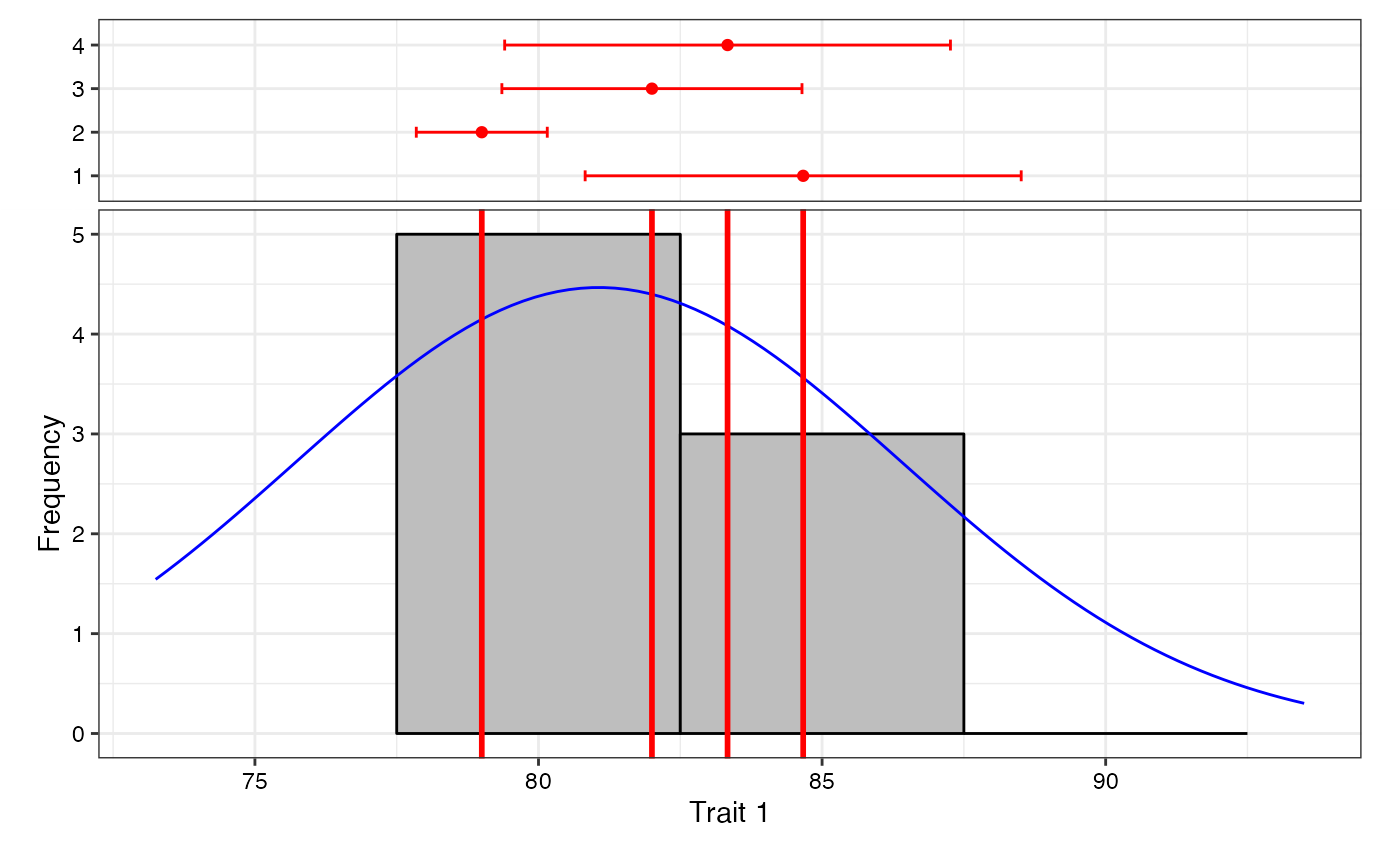
# Frequency distribution plots
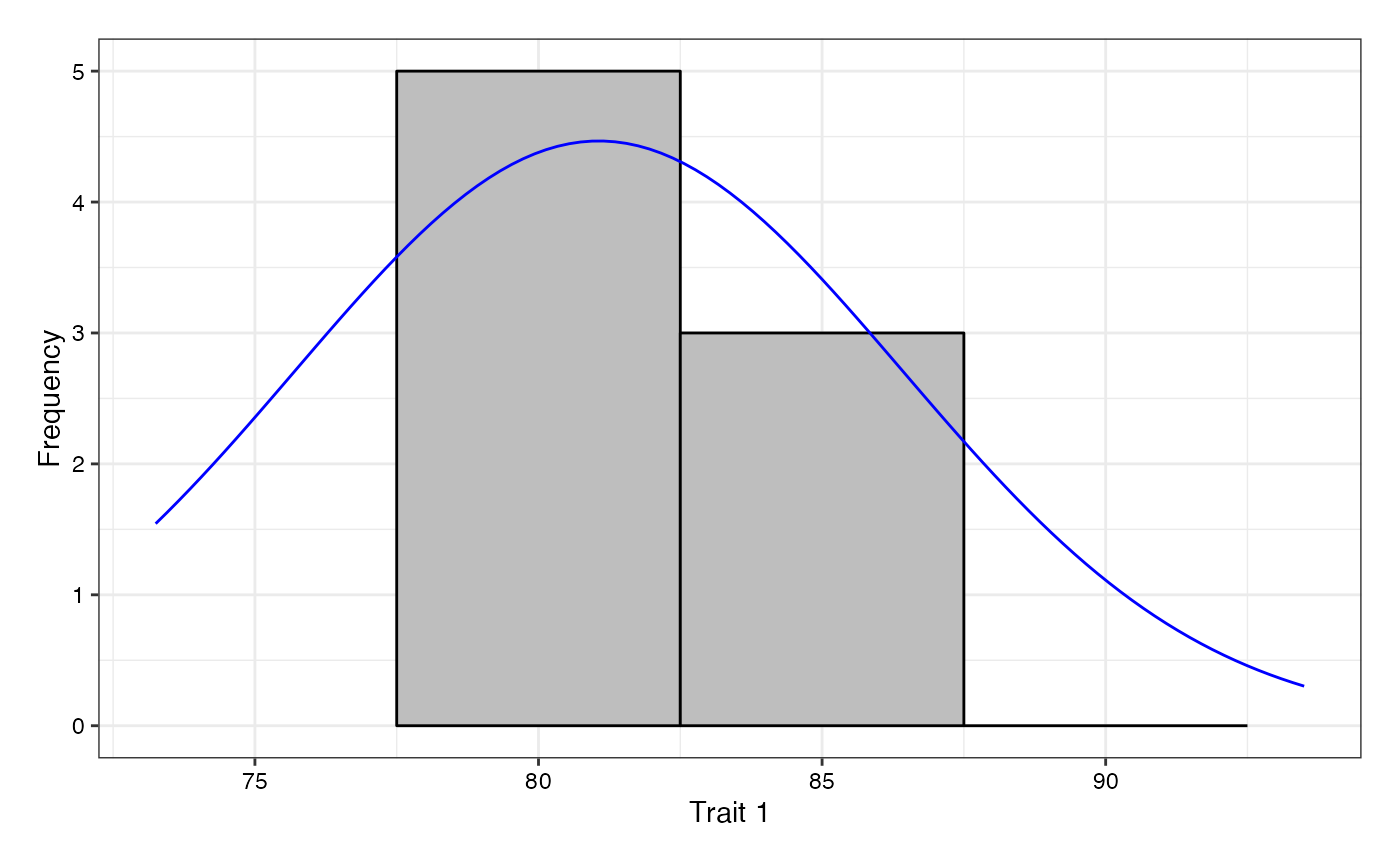
freq1 <- freqdist.augmentedRCBD(out1, xlab = "Trait 1")
#> Warning: Removed 2 rows containing missing values or values outside the scale range
#> (`geom_bar()`).
class(freq1)
#> [1] "gtable" "gTree" "grob" "gDesc"
plot(freq1)
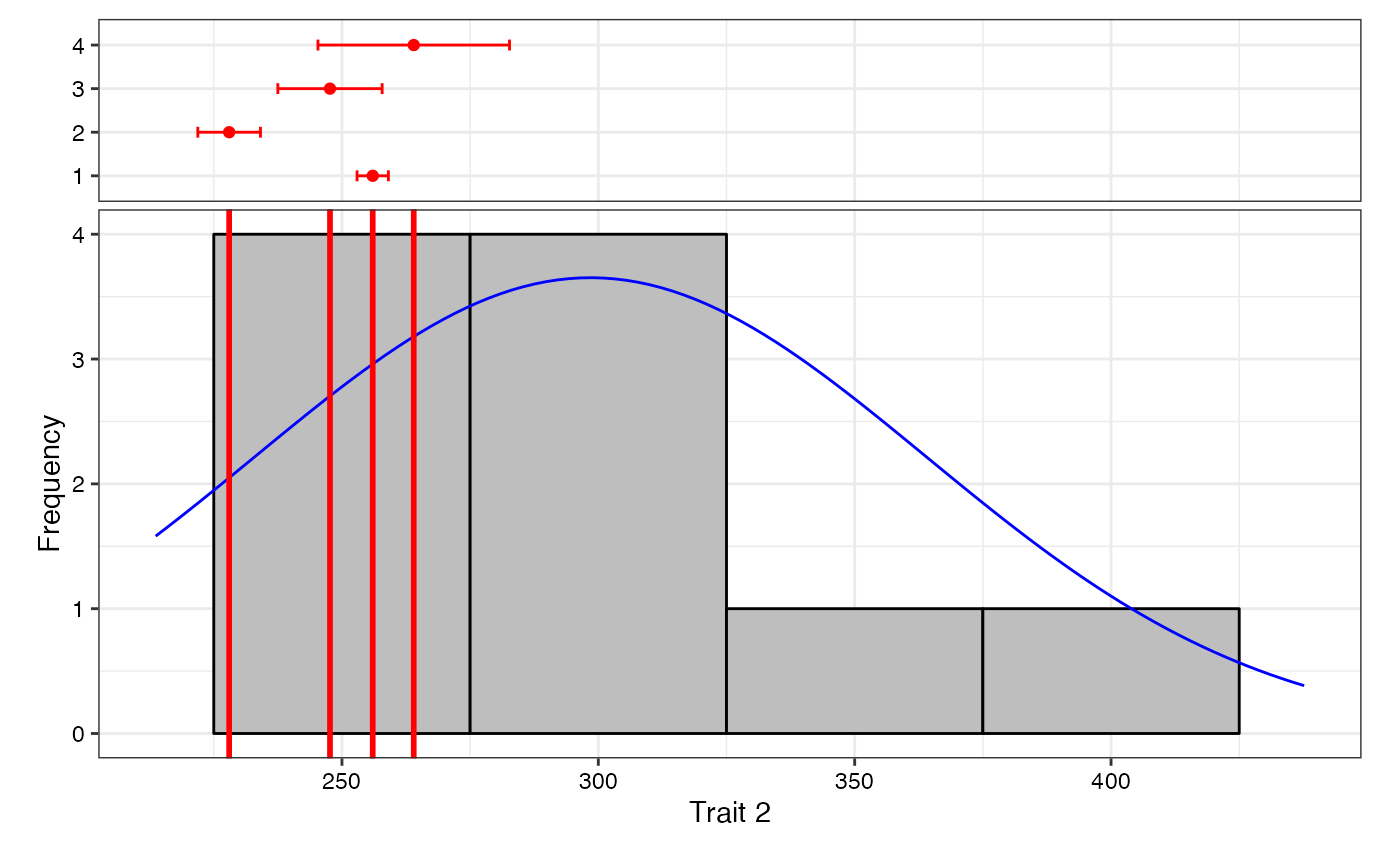
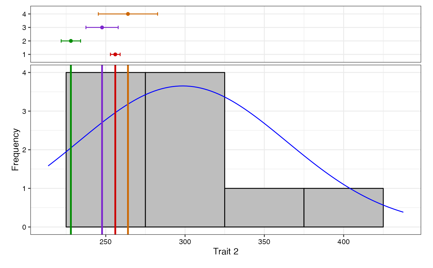
 freq2 <- freqdist.augmentedRCBD(out2, xlab = "Trait 2")
#> Warning: Removed 2 rows containing missing values or values outside the scale range
#> (`geom_bar()`).
plot(freq2)
freq2 <- freqdist.augmentedRCBD(out2, xlab = "Trait 2")
#> Warning: Removed 2 rows containing missing values or values outside the scale range
#> (`geom_bar()`).
plot(freq2)
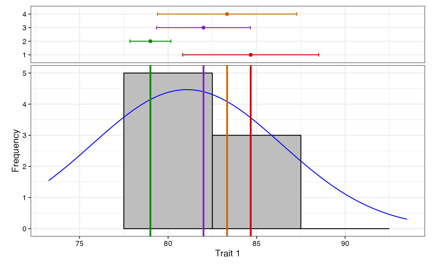
 # Change check colours
colset <- c("red3", "green4", "purple3", "darkorange3")
freq1 <- freqdist.augmentedRCBD(out1, xlab = "Trait 1", check.col = colset)
#> Warning: Removed 2 rows containing missing values or values outside the scale range
#> (`geom_bar()`).
plot(freq1)
# Change check colours
colset <- c("red3", "green4", "purple3", "darkorange3")
freq1 <- freqdist.augmentedRCBD(out1, xlab = "Trait 1", check.col = colset)
#> Warning: Removed 2 rows containing missing values or values outside the scale range
#> (`geom_bar()`).
plot(freq1)
 freq2 <- freqdist.augmentedRCBD(out2, xlab = "Trait 2", check.col = colset)
#> Warning: Removed 2 rows containing missing values or values outside the scale range
#> (`geom_bar()`).
plot(freq2)
freq2 <- freqdist.augmentedRCBD(out2, xlab = "Trait 2", check.col = colset)
#> Warning: Removed 2 rows containing missing values or values outside the scale range
#> (`geom_bar()`).
plot(freq2)
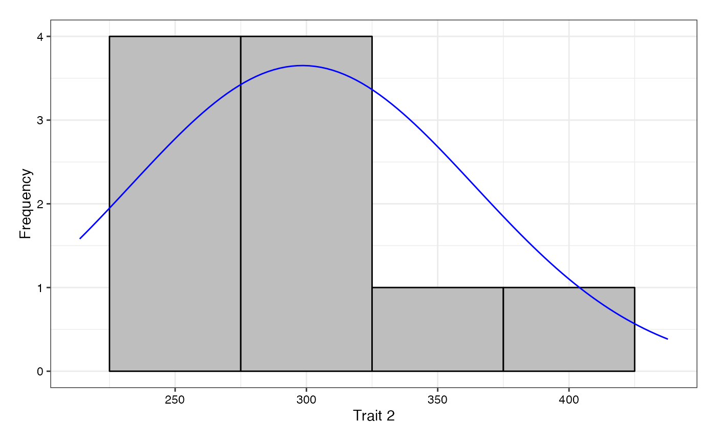
 # Without checks highlighted
freq1 <- freqdist.augmentedRCBD(out1, xlab = "Trait 1",
highlight.check = FALSE)
#> Warning: Removed 2 rows containing missing values or values outside the scale range
#> (`geom_bar()`).
plot(freq1)
# Without checks highlighted
freq1 <- freqdist.augmentedRCBD(out1, xlab = "Trait 1",
highlight.check = FALSE)
#> Warning: Removed 2 rows containing missing values or values outside the scale range
#> (`geom_bar()`).
plot(freq1)
 freq2 <- freqdist.augmentedRCBD(out2, xlab = "Trait 2",
highlight.check = FALSE)
#> Warning: Removed 2 rows containing missing values or values outside the scale range
#> (`geom_bar()`).
plot(freq2)
freq2 <- freqdist.augmentedRCBD(out2, xlab = "Trait 2",
highlight.check = FALSE)
#> Warning: Removed 2 rows containing missing values or values outside the scale range
#> (`geom_bar()`).
plot(freq2)