Data Analysis with `augmentedRCBD`
Aravind, J.1, Mukesh Sankar, S.2, Wankhede, D. P.3, and Kaur, V.4
2026-04-28
Source:vignettes/Data_Analysis_with_augmentedRCBD.Rmd
Data_Analysis_with_augmentedRCBD.Rmd
- Division of Germplasm Conservation, ICAR-National Bureau of Plant Genetic Resources, New Delhi.
- Division of Genetics, ICAR-Indian Agricultural Research Institute, New Delhi.
- Division of Genomic Resources, ICAR-National Bureau of Plant Genetic Resources, New Delhi.
- Division of Germplasm Evaluation, ICAR-National Bureau of Plant Genetic Resources, New Delhi.

1 Overview
The software augmentedRCBD is built on the R
statistical programming language as an add-on (or ‘package’ in the
R lingua franca). It performs the analysis of data
generated from experiments in augmented randomised complete block design
according to Federer, W.T. (1956a, 1956b, 1961; 1976). It
also computes analysis of variance, adjusted means, descriptive
statistics, genetic variability statistics etc. and includes options for
data visualization and report generation.
This tutorial aims to educate the users in utilising this package for
performing such analysis. Utilising augmentedRCBD for data
analysis requires a basic knowledge of R programming
language. However, as many of the intended end-users may not be familiar
with R, sections 2 to 4 give a
‘gentle’ introduction to R, especially those aspects which
are necessary to get augmentedRCBD up and running for
performing data analysis in a Windows environment. Users already
familiar with R can feel free to skip to section 5.
![]()
2 R software
It is a free software environment for statistical computing and graphics. It is free and open source, platform independent (works on Linux, Windows or MacOS), very flexible, comprehensive with robust interfaces for all the popular programming languages as well as databases. It is strengthened by its diverse library of add-on packages extending its ability as well as the incredible community support. It is one of the most popular tools being used in academia today (Tippmann, 2015).
3 Getting Started
This section details the steps required to set up the R
programming environment under a third-party interface called
RStudio in Windows.
3.1 Installing R
Download and install R for Windows from http://cran.r-project.org/bin/windows/base/.

Fig. 1: The R download location.
3.2 Installing RStudio
The basic command line
interface in native R is rather limiting. There are
several interfaces which enhance it’s functionality and ease of use, RStudio being one of
the most popular among R programmers.
Download and install RStudio for Windows from https://www.rstudio.com/products/rstudio/download/#download

Fig. 2: The RStudio download location.
3.3 The RStudio Interface
On opening RStudio, the default interface with four
panes/windows is visible as follows. Few panes have different tabs.

Fig. 3: The default RStudio interface with
the four panes.
3.3.1 Console
This is where the action happens. Here any authentic R
code typed after the ‘>’ prompt will be executed after
pressing ‘Enter’ to generate the output.
For example, type 1+1 in the console and press
‘Enter’.
1+1[1] 23.3.2 Source
This is where R Scripts (collection of code) can be
created and edited. R scripts are text files with a
.R extension. R Code for analysis can be typed
and saved in such R scripts. New scripts can be opened by
clicking ‘File|New File’ and selecting ‘R Script’. Code can be selected
from R Scripts and sent to console for evaluation by
clicking ‘Run’ on the ‘Source’ pane or by pressing ‘Ctrl + Enter’.
3.3.3 Environment|History|Connections
The ‘Environment’ tab shows the list of all the ‘objects’ (see section 4.3) defined in the current R
session. It has also some buttons up top to open, save and clear the
environment as well as few options for import of data under
Import Dataset.
The ‘History’ tab shows a history of all the code that was previously evaluated. This is useful, if you want to go back to some code.
The ‘Connections’ tab helps to establish and manage connections with different databases and data sources.
3.3.4 Files|Plots|Packages|Help|Viewer
The ‘Files’ tab shows a sleek file browser to access the file directory in the computer with options to manage the working directory (see section 4.1) under the More button.
The ‘Plots’ tab shows all the plots generated in R with
buttons to delete unnecessary ones and export useful ones as a pdf file
or as an image file.
The ‘Packages’ tab shows a list of all the R add-on
packages installed. The check box on the left shows whether they are
loaded or not. There are also buttons to install and update
R packages.
The ‘Viewer’ tab shows any web content output generated by an
R code.
4 Some Basics
This section describes some basics to enable the users to have a
working knowledge in R in order to use
augmentedRCBD.
4.1 Working Directory
It is a file path to a folder on the computer which is recognised by
R as the default location to read files from or write files
to. The code getwd() shows the current working directory,
while setwd() can be used to change the existing working
directory.
# Print current working directory
getwd()
[1] "C:/Users/Computer/Documents"[1] "C:/Data Analysis/"One key detail is that file paths in R uses forward
slashes (/) as in MacOS or Linux, unlike backward slashes
(\) in Windows. This needs to be considered while copying
paths from default Windows file explorer.
4.2 Expression and Assignment
Expressions are instructions in the form of code to be entered after
the > prompt in the console. Expressions can be a
constant, an arithmetic or a condition. A more advanced and most useful
expression is a function call (see section
4.3).
# Constant
123
[1] 123
# Arithmetic (add two numbers)
1 + 2
[1] 3
# Condition
34 > 25
[1] TRUE
1 == 2[1] FALSE[1] 51.25Information from an expression can be stored as an ‘object’ (see section 4.3) by assigning a name using the operator
‘<-’.
# Assign the result of the expression 1 + 2 to an object 'a'
a <- 1 + 2
a
[1] 3It is recommended to add comments to explain the code by using the
‘#’ sign. Any code after the ‘#’ sign will be
ignored by R.
4.3 Objects and Functions
R is an object-oriented programming language (OOP). Any
kind or construct created in R is an ‘object’. Each object
has a ‘class’ (shown using the class() function) and
different ‘attributes’ which defines what operations can be done on that
object. There are different types of data structure objects in
R such as vectors, matrices, factors, data frames, and
lists. A ‘function’ is also an object, which defines a procedure or a
sequence of expressions.
4.3.1 Vector
A vector is a collection of elements of a single type (or ‘mode’).
The common vector modes are ‘numeric’, ‘integer’, ‘character’ and
‘logical’. The c() function is used to create vectors. The
functions class(), str() and
length() show the attributes of vectors.
Vector modes ‘numeric’ stores real numbers, while ‘integer’ stores
integers, which can be enforced by suffixing elements with
‘L’.
[1] "numeric"
str(a) num [1:3] 1 2 3.3
length(a)[1] 3[1] "integer"
str(b) int [1:3] 1 2 3
length(b)[1] 3The vector mode ‘character’ store text.
[1] "character"
str(c) chr [1:3] "one" "two" "three"
length(c)[1] 3The vector mode ‘logical’ stores ‘TRUE’ OR
‘FALSE’ logical data.
[1] "logical"
str(d) logi [1:6] TRUE TRUE TRUE FALSE TRUE FALSE
length(d)[1] 64.3.2 Factor
A ‘factor’ in R stores data from categorical data in
variables as different levels.
catg <- c("male","female","female","male","male")
catg
[1] "male" "female" "female" "male" "male"
is.factor(catg)[1] FALSE
# Apply the factor function
factor_catg <- factor(catg)

factor_catg
[1] male female female male male
Levels: female male
is.factor(factor_catg)[1] TRUE
class(factor_catg)[1] "factor"
str(factor_catg) Factor w/ 2 levels "female","male": 2 1 1 2 2A character, numeric or integer vector can be transformed to a factor
by using the as.factor() function.
[1] "numeric"
str(a) num [1:3] 1 2 3.3[1] "factor"
str(fac_a) Factor w/ 3 levels "1","2","3.3": 1 2 3[1] "integer"
str(b) int [1:3] 1 2 3[1] "factor"
str(fac_b) Factor w/ 3 levels "1","2","3": 1 2 3[1] "character"
str(c) chr [1:3] "one" "two" "three"[1] "factor"
str(fac_c) Factor w/ 3 levels "one","three",..: 1 3 24.3.3 Matrix
A ‘matrix’ in R is a vector with the attributes
‘nrow’ and ‘ncol’.
# Generate 5 * 4 numeric matrix
m <- matrix(1:20, nrow = 5, ncol = 4)
m
[,1] [,2] [,3] [,4]
[1,] 1 6 11 16
[2,] 2 7 12 17
[3,] 3 8 13 18
[4,] 4 9 14 19
[5,] 5 10 15 20
class(m)[1] "matrix" "array"
typeof(m)[1] "integer"
# Dimensions of m
dim(m)
[1] 5 44.3.4 List
A ‘list’ is a container containing different objects. The contents of list need not be of the same type or mode. A list can encompass a mixture of data types such as vectors, matrices, data frames, other lists or any other data structure.
[1] "list"
str(w)List of 4
$ : num [1:3] 1 2 3.3
$ : int [1:5, 1:4] 1 2 3 4 5 6 7 8 9 10 ...
$ : logi [1:6] TRUE TRUE TRUE FALSE TRUE FALSE
$ :List of 2
..$ : int [1:3] 1 2 3
..$ : chr [1:3] "one" "two" "three"4.3.5 Data Frame
A ‘data frame’ in R is a special kind of list with every
element having equal length. It is very important for handling tabular
data in R. It is a array like structure with rows and
columns. Each column needs to be of a single data type, however data
type can vary between columns.
L <- LETTERS[1:4]
y <- 1:4
z <- c("This", "is", "a", "data frame")
df <- data.frame(L, x = 1, y, z)
df
L x y z
1 A 1 1 This
2 B 1 2 is
3 C 1 3 a
4 D 1 4 data frame
str(df)'data.frame': 4 obs. of 4 variables:
$ L: chr "A" "B" "C" "D"
$ x: num 1 1 1 1
$ y: int 1 2 3 4
$ z: chr "This" "is" "a" "data frame"
attributes(df)$names
[1] "L" "x" "y" "z"
$class
[1] "data.frame"
$row.names
[1] 1 2 3 4
rownames(df)[1] "1" "2" "3" "4"
colnames(df)[1] "L" "x" "y" "z"4.3.6 Functions
All of the work in R is done by functions. It is an
object defining a procedure which takes one or more objects as input (or
‘arguments’), performs some action on them and finally gives a new
object as output (or ‘return’). class(),
mean(), getwd(), +, etc. are all
functions.
For example the function mean() takes a numeric vector
as argument and returns the mean as a numeric vector.
[1] 2.1The user can also create custom functions. For example the function
foo adds two numbers and gives the result.
foo <- function(n1, n2) {
  out <- n1 + n2
  return(out)
}
foo(2,3)
[1] 54.4 Special Elements
In addition to numbers and text, there are some special elements which can be included in different data objects.
NA (not available) indicates missing data.
[1] FALSE TRUE FALSE
is.na(z)[1] FALSE TRUE FALSE FALSE FALSE
anyNA(x)[1] TRUE
a[1] 1.0 2.0 3.3
is.na(a)[1] FALSE FALSE FALSEInf indicates infinity.
1/0[1] InfNaN (Not a Number) indicates any undefined value.
0/0[1] NaN4.5 Indexing
The [ function is used to extract elements of an object
by indexing (numeric or logical). Named elements in lists and data
frames can be extracted by using the $ operator.
Consider a vector a.
a <- c(1, 2, 3.3, 2.8, 6.7)
# Numeric indexing
# Extract first element
a[1]
[1] 1
# Extract elements 2:3
a[2:3]
[1] 2.0 3.3
# Logical indexing
a[a > 3]
[1] 3.3 6.7Consider a matrix m.
     a b c
[1,] 1 2 3
[2,] 4 5 6
[3,] 7 8 9
# Extract elements
m[,2] # 2nd column of matrix
[1] 2 5 8
m[3,] # 3rd row of matrixa b c
7 8 9
m[2:3, 1:3] # rows 2,3 of columns 1,2,3 a b c
[1,] 4 5 6
[2,] 7 8 9
m[2,2] # Element in 2nd column of 2nd rowb
5
m[, 'b'] # Column 'b'[1] 2 5 8
m[, c('a', 'c')] # Column 'a' and 'c' a c
[1,] 1 3
[2,] 4 6
[3,] 7 9Consider a list w.
w <- list(vec = a, mat = m, data = df, alist = list(b, c))

# Indexing by number
w[2] # As list structure
$mat
     a b c
[1,] 1 2 3
[2,] 4 5 6
[3,] 7 8 9
w[[2]] # Without list structure a b c
[1,] 1 2 3
[2,] 4 5 6
[3,] 7 8 9
# Indexing by name
w$vec
[1] 1.0 2.0 3.3 2.8 6.7
w$data L x y z
1 A 1 1 This
2 B 1 2 is
3 C 1 3 a
4 D 1 4 data frameConsider a data frame df.
df L x y z
1 A 1 1 This
2 B 1 2 is
3 C 1 3 a
4 D 1 4 data frame
# Indexing by number
df[,2] # 2nd column of data frame
[1] 1 1 1 1
df[2] # 2nd column of data frame x
1 1
2 1
3 1
4 1
df[3,] # 3rd row of data frame L x y z
3 C 1 3 a
df[2:3, 1:3] # rows 2,3 of columns 1,2,3 L x y
2 B 1 2
3 C 1 3
df[2,2] # Element in 2nd column of 2nd row[1] 1
# Indexing by name
df$L
[1] "A" "B" "C" "D"
df$z[1] "This" "is" "a" "data frame"4.6 Help Documentation
The help documentation regarding any function can be viewed using the
? or help() function. The help documentation
shows the default usage of the function including, the arguments that
are taken by the function and the type of output object returned
(‘Value’).
?ls
help(ls)

?mean

?setwd
4.7 Packages
Packages in R are collections of R
functions, data, and compiled code in a well-defined format. They are
add-ons which extend the functionality of R and at present,
there are 23717
packages available for deployment and use at the official repository,
the Comprehensive R Archive Network (CRAN).
Valid packages from CRAN can be installed by using the
install.packages() command.
# Install the package 'readxl' for importing data from excel
install.packages(readxl)
Installed packages can be loaded using the function
library().
4.8 Importing and Exporting Tabular Data
Tabular data from a spreadsheet can be imported into R
in different ways. Consider some data such as in Table 1. Copy this data
in to a spreadsheet editor such as MS Excel and save it as
augdata.csv, a comma-separated-value file and
augdata.xlsx, an Excel file in the working directory
(getwd()).
Table 1: Example data from an experiment in augmented RCBD design.
| blk | trt | y1 | y2 |
|---|---|---|---|
| I | 1 | 92 | 258 |
| I | 2 | 79 | 224 |
| I | 3 | 87 | 238 |
| I | 4 | 81 | 278 |
| I | 7 | 96 | 347 |
| I | 11 | 89 | 300 |
| I | 12 | 82 | 289 |
| II | 1 | 79 | 260 |
| II | 2 | 81 | 220 |
| II | 3 | 81 | 237 |
| II | 4 | 91 | 227 |
| II | 5 | 79 | 281 |
| II | 9 | 78 | 311 |
| III | 1 | 83 | 250 |
| III | 2 | 77 | 240 |
| III | 3 | 78 | 268 |
| III | 4 | 78 | 287 |
| III | 8 | 70 | 226 |
| III | 6 | 75 | 395 |
| III | 10 | 74 | 450 |
The augdata.csv file can be imported into R
using the read.csv() function or the read_csv()
function in the readr package.
'data.frame':   20 obs. of  4 variables:
 $ blk: Factor w/ 3 levels "I","II","III": 1 1 1 1 1 1 1 2 2 2 ...
 $ trt: num  1 2 3 4 7 11 12 1 2 3 ...
 $ y1 : num  92 79 87 81 96 89 82 79 81 81 ...
 $ y2 : num  258 224 238 278 347 300 289 260 220 237 ...
The argument stringsAsFactors = FALSE reads the text
columns as of type character instead of the default
factor.
'data.frame':   20 obs. of  4 variables:
 $ blk: chr  "I" "I" "I" "I" ...
 $ trt: num  1 2 3 4 7 11 12 1 2 3 ...
 $ y1 : num  92 79 87 81 96 89 82 79 81 81 ...
 $ y2 : num  258 224 238 278 347 300 289 260 220 237 ...
The augdata.xlsx file can be imported into
R using the read_excel()
function in the readxl package.
library(readxl)
data <- read_excel(path = "augdata.xlsx")
'data.frame': 20 obs. of 4 variables:
$ blk: chr "I" "I" "I" "I" ...
$ trt: num 1 2 3 4 7 11 12 1 2 3 ...
$ y1 : num 92 79 87 81 96 89 82 79 81 81 ...
$ y2 : num 258 224 238 278 347 300 289 260 220 237 ...The tabular data can be exported from R to a
.csv (comma-separated-value) file by the write.csv()
function.
write.csv(x = data, file = "augdata.csv")4.9 Additional Resources
To learn more about R, there are umpteen number of
online tutorials as well as free courses available. Queries about
various aspects can be put to the active and vibrant `R community
online.
- Online tutorials
- Free online courses
-
Rcommunity support- http://stackoverflow.com/
-
Rhelp mailing lists : http://www.r-project.org/mail.html
5 Installation of augmentedRCBD
The package augmentedRCBD can be installed using the
following functions.
# Install from CRAN
install.packages('augmentedRCBD', dependencies=TRUE)

# Install development version from Github
if (!require('devtools')) install.packages('devtools')
library(devtools)
install_github("aravind-j/augmentedRCBD")
The stable release is hosted in CRAN (see section 4.7), while the under-development version
is hosted as a Github repository.
To install from github, you need to use the install_github()
function from `devtools
package.
Then the package can be loaded using the function
--------------------------------------------------------------------------------
Welcome to augmentedRCBD version 0.1.7.9000


# To know how to use this package type:
  browseVignettes(package = 'augmentedRCBD')
  for the package vignette.

# To know whats new in this version type:
  news(package='augmentedRCBD')
  for the NEWS file.

# To cite the methods in the package type:
  citation(package='augmentedRCBD')

# To suppress this message use:
  suppressPackageStartupMessages(library(augmentedRCBD))
--------------------------------------------------------------------------------
The current version of the package is 0.1.7.9000. The previous versions are as follows.
Table 2. Version history of
augmentedRCBD R package.
| Version | Date |
|---|---|
| 0.1.0 | 2018-07-10 |
| 0.1.1 | 2019-07-21 |
| 0.1.2 | 2020-03-19 |
| 0.1.3 | 2020-07-27 |
| 0.1.4 | 2021-02-17 |
| 0.1.5 | 2021-06-12 |
| 0.1.6 | 2023-05-28 |
| 0.1.7 | 2023-08-19 |
To know detailed history of changes use
news(package='augmentedRCBD').
6 Data Format
Certain details need to be considered for arranging experimental data
for analysis using the augmentedRCBD package.
The data should be in long/vertical form, where each row has the data from one genotype per block. For example, consider the following data (Table 3) recorded for a trait from an experiment laid out in an augmented block design with 3 blocks and 12 genotypes(or treatment) with 6 to 7 genotypes/block. 8 genotypes (Test, G 5 to G 12) are not replicated, while 4 genotypes (Check, G 1 to G 4) are replicated.
Table 3: Data from an experiment in augmented RCBD design.
| Block I | G12 | G4 | G11 | G2 | G1 | G7 | G3 |
| 82 | 81 | 89 | 79 | 92 | 96 | 87 | |
| Block II | G5 | G9 | – | G3 | G1 | G2 | G4 |
| 79 | 78 | – | 81 | 79 | 81 | 91 | |
| Block III | G4 | G2 | G1 | G6 | G10 | G3 | G8 |
| 78 | 77 | 83 | 75 | 74 | 78 | 70 |
This data needs to be arranged with columns showing block, genotype (or treatment) and the data of the trait for each genotype per block (Table 4).
Table 4: Data from an experiment in augmented RCBD design arranged in long-form.
| Block | Treatment | Trait |
|---|---|---|
| Block I | G 1 | 92 |
| Block I | G 2 | 79 |
| Block I | G 3 | 87 |
| Block I | G 4 | 81 |
| Block I | G 7 | 96 |
| Block I | G 11 | 89 |
| Block I | G 12 | 82 |
| Block II | G 1 | 79 |
| Block II | G 2 | 81 |
| Block II | G 3 | 81 |
| Block II | G 4 | 91 |
| Block II | G 5 | 79 |
| Block II | G 9 | 78 |
| Block III | G 1 | 83 |
| Block III | G 2 | 77 |
| Block III | G 3 | 78 |
| Block III | G 4 | 78 |
| Block III | G 8 | 70 |
| Block III | G 6 | 75 |
| Block III | G 10 | 74 |
The data for block and genotype (or treatment) can also be depicted as numbers (Table 5).
Table 5: Data from an experiment in augmented RCBD design arranged in long-form (Block and Treatment as numbers).
| Block | Treatment | Trait |
|---|---|---|
| 1 | 1 | 92 |
| 1 | 2 | 79 |
| 1 | 3 | 87 |
| 1 | 4 | 81 |
| 1 | 7 | 96 |
| 1 | 11 | 89 |
| 1 | 12 | 82 |
| 2 | 1 | 79 |
| 2 | 2 | 81 |
| 2 | 3 | 81 |
| 2 | 4 | 91 |
| 2 | 5 | 79 |
| 2 | 9 | 78 |
| 3 | 1 | 83 |
| 3 | 2 | 77 |
| 3 | 3 | 78 |
| 3 | 4 | 78 |
| 3 | 8 | 70 |
| 3 | 6 | 75 |
| 3 | 10 | 74 |
Multiple traits can be added as additional columns (Table 6).
Table 6: Data from an experiment in augmented RCBD design arranged in long-form (Multiple traits).
| Block | Treatment | Trait1 | Trait2 |
|---|---|---|---|
| Block I | G 1 | 92 | 258 |
| Block I | G 2 | 79 | 224 |
| Block I | G 3 | 87 | 238 |
| Block I | G 4 | 81 | 278 |
| Block I | G 7 | 96 | 347 |
| Block I | G 11 | 89 | 300 |
| Block I | G 12 | 82 | 289 |
| Block II | G 1 | 79 | 260 |
| Block II | G 2 | 81 | 220 |
| Block II | G 3 | 81 | 237 |
| Block II | G 4 | 91 | 227 |
| Block II | G 5 | 79 | 281 |
| Block II | G 9 | 78 | 311 |
| Block III | G 1 | 83 | 250 |
| Block III | G 2 | 77 | 240 |
| Block III | G 3 | 78 | 268 |
| Block III | G 4 | 78 | 287 |
| Block III | G 8 | 70 | 226 |
| Block III | G 6 | 75 | 395 |
| Block III | G 10 | 74 | 450 |
Data should preferably be balanced i.e. all the check genotypes should be present in all the blocks. If not, a warning is issued. The number of test genotypes can vary within a block. There should not be any missing values. Rows of genotypes with missing values for one or more traits should be removed.
Such a tabular data should be imported (see section
7.8) into R as a data frame object (see section 4.3.5). The columns with the block and
treatment categorical data should of the type factor (see section 4.3.2), while the column(s) with the
trait data should be of the type integer or numeric (see section 4.3.1).
7 Data Analysis for a Single Trait
Analysis of data for a single trait can be performed by using
augmentedRCBD function. It generates an object of class
augmentedRCBD. Such an object can then be taken as input by
the several functions to print the results to console
(print.augmentedRCBD), generate descriptive statistics from
adjusted means (describe.augmentedRCBD), plot frequency
distribution (freqdist.augmentedRCBD) and computed genetic
variability statistics (gva.augmentedRCBD). All these outputs can also
be exported as a MS Word report using the
report.augmentedRCBD function.
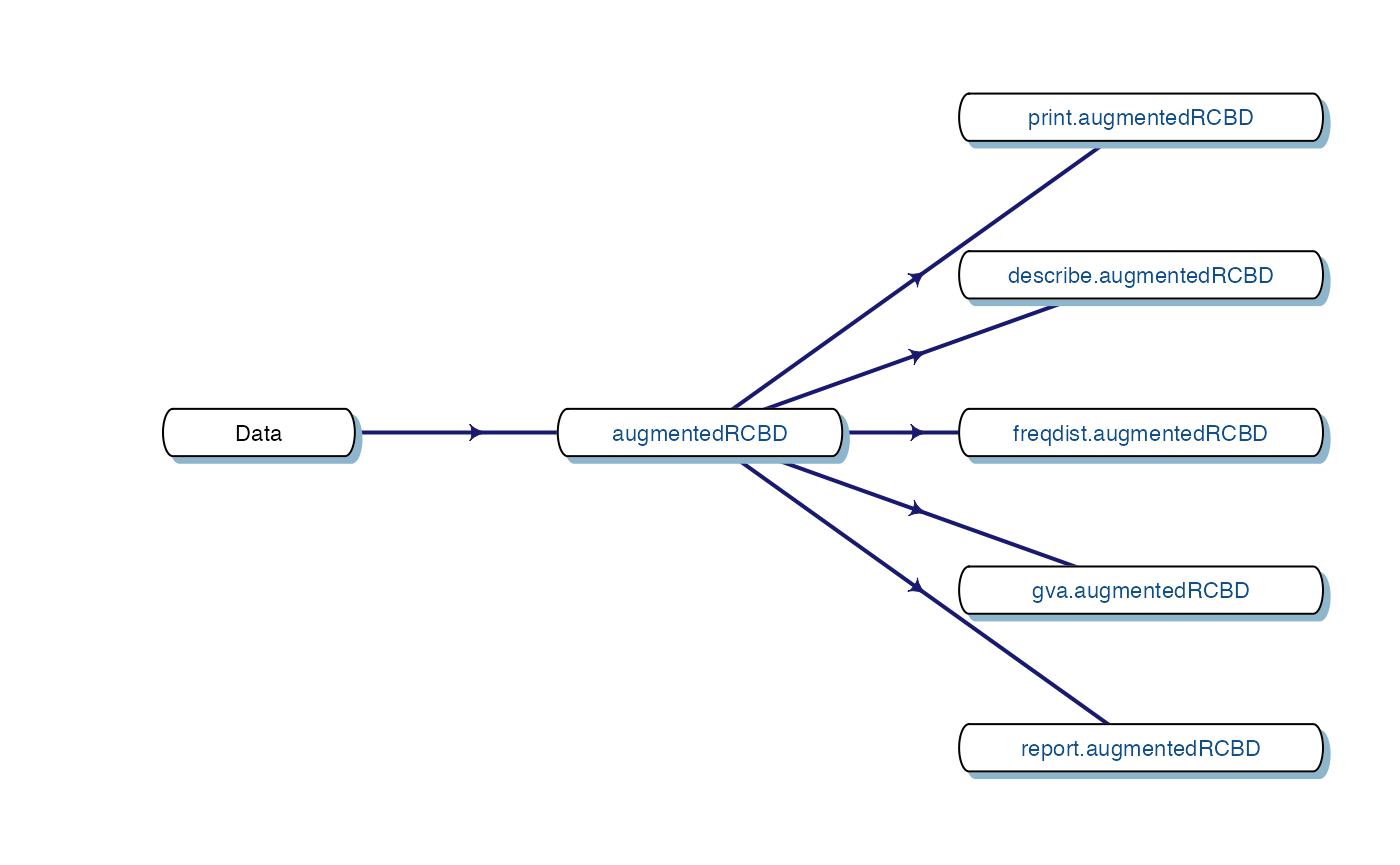
Fig. 4. Workflow for analysis of single traits with
augmentedRCBD.
7.1 augmentedRCBD()
Consider the data in Table 1. The data can be
imported into R as vectors as
follows.
blk <- c(1, 1, 1, 1, 1, 1, 1, 2, 2, 2, 2, 2, 2, 3, 3, 3, 3, 3, 3, 3)
trt <- c(1, 2, 3, 4, 7, 11, 12, 1, 2, 3, 4, 5, 9, 1, 2, 3, 4, 8, 6, 10)
y1 <- c(92, 79, 87, 81, 96, 89, 82, 79, 81, 81, 91, 79, 78, 83, 77, 78, 78,
        70, 75, 74)
y2 <- c(258, 224, 238, 278, 347, 300, 289, 260, 220, 237, 227, 281, 311, 250,
        240, 268, 287, 226, 395, 450)
The blk and trt vectors with the block and
treatment data need to be converted into factors as follows before
analysis.
With the data in appropriate format, the analysis can be performed as
follows for the trait y1 as follows.
out1 <- augmentedRCBD(blk, trt, y1, method.comp = "lsd",
                      alpha = 0.05, group = TRUE, console = TRUE)
Augmented Design Details
========================

Number of blocks           "3"
Number of treatments       "12"
Number of check treatments "4"
Number of test treatments  "8"
Check treatments           "1, 2, 3, 4"


ANOVA, Treatment Adjusted
=========================
                                     Df Sum Sq Mean Sq F value Pr(>F)
Block (ignoring Treatments)           2  360.1  180.04   6.675 0.0298 *
Treatment (eliminating Blocks)       11  285.1   25.92   0.961 0.5499
  Treatment: Check                    3   52.9   17.64   0.654 0.6092
  Treatment: Test and Test vs. Check  8  232.2   29.02   1.076 0.4779
Residuals                             6  161.8   26.97
---
Signif. codes:  0 '***' 0.001 '**' 0.01 '*' 0.05 '.' 0.1 ' ' 1

ANOVA, Block Adjusted
=====================
                               Df Sum Sq Mean Sq F value Pr(>F)
Treatment (ignoring Blocks)    11  575.7   52.33   1.940  0.215
  Treatment: Check              3   52.9   17.64   0.654  0.609
  Treatment: Test               7  505.9   72.27   2.679  0.125
  Treatment: Test vs. Check     1   16.9   16.87   0.626  0.459
Block (eliminating Treatments)  2   69.5   34.75   1.288  0.342
Residuals                       6  161.8   26.97

Coefficient of Variation
========================
6.372367

Overall Adjusted Mean
=====================
81.0625

Standard Errors
===============
                                         Std. Error of Diff.  CD (5%)
Control Treatment Means                             4.240458 10.37603
Two Test Treatments (Same Block)                    7.344688 17.97180
Two Test Treatments (Different Blocks)              8.211611 20.09309
A Test Treatment and a Control Treatment            6.704752 16.40594

Treatment Means
===============
 Treatment Block Means   SE r   Min   Max Adjusted Means
         1       84.67 3.84 3 79.00 92.00          84.67
        10     3 74.00 <NA> 1 74.00 74.00          77.25
        11     1 89.00 <NA> 1 89.00 89.00          86.50
        12     1 82.00 <NA> 1 82.00 82.00          79.50
         2       79.00 1.15 3 77.00 81.00          79.00
         3       82.00 2.65 3 78.00 87.00          82.00
         4       83.33 3.93 3 78.00 91.00          83.33
         5     2 79.00 <NA> 1 79.00 79.00          78.25
         6     3 75.00 <NA> 1 75.00 75.00          78.25
         7     1 96.00 <NA> 1 96.00 96.00          93.50
         8     3 70.00 <NA> 1 70.00 70.00          73.25
         9     2 78.00 <NA> 1 78.00 78.00          77.25


Comparisons
===========

Method : lsd

                  contrast estimate   SE df t.ratio p.value sig
   treatment1 - treatment2     5.67 4.24  6   1.336   0.230
   treatment1 - treatment3     2.67 4.24  6   0.629   0.553
   treatment1 - treatment4     1.33 4.24  6   0.314   0.764
   treatment1 - treatment5     6.42 6.36  6   1.009   0.352
   treatment1 - treatment6     6.42 6.36  6   1.009   0.352
   treatment1 - treatment7    -8.83 6.36  6  -1.389   0.214
   treatment1 - treatment8    11.42 6.36  6   1.795   0.123
   treatment1 - treatment9     7.42 6.36  6   1.166   0.288
  treatment1 - treatment10     7.42 6.36  6   1.166   0.288
  treatment1 - treatment11    -1.83 6.36  6  -0.288   0.783
  treatment1 - treatment12     5.17 6.36  6   0.812   0.448
   treatment2 - treatment3    -3.00 4.24  6  -0.707   0.506
   treatment2 - treatment4    -4.33 4.24  6  -1.022   0.346
   treatment2 - treatment5     0.75 6.36  6   0.118   0.910
   treatment2 - treatment6     0.75 6.36  6   0.118   0.910
   treatment2 - treatment7   -14.50 6.36  6  -2.280   0.063
   treatment2 - treatment8     5.75 6.36  6   0.904   0.401
   treatment2 - treatment9     1.75 6.36  6   0.275   0.792
  treatment2 - treatment10     1.75 6.36  6   0.275   0.792
  treatment2 - treatment11    -7.50 6.36  6  -1.179   0.283
  treatment2 - treatment12    -0.50 6.36  6  -0.079   0.940
   treatment3 - treatment4    -1.33 4.24  6  -0.314   0.764
   treatment3 - treatment5     3.75 6.36  6   0.590   0.577
   treatment3 - treatment6     3.75 6.36  6   0.590   0.577
   treatment3 - treatment7   -11.50 6.36  6  -1.808   0.121
   treatment3 - treatment8     8.75 6.36  6   1.376   0.218
   treatment3 - treatment9     4.75 6.36  6   0.747   0.483
  treatment3 - treatment10     4.75 6.36  6   0.747   0.483
  treatment3 - treatment11    -4.50 6.36  6  -0.707   0.506
  treatment3 - treatment12     2.50 6.36  6   0.393   0.708
   treatment4 - treatment5     5.08 6.36  6   0.799   0.455
   treatment4 - treatment6     5.08 6.36  6   0.799   0.455
   treatment4 - treatment7   -10.17 6.36  6  -1.598   0.161
   treatment4 - treatment8    10.08 6.36  6   1.585   0.164
   treatment4 - treatment9     6.08 6.36  6   0.956   0.376
  treatment4 - treatment10     6.08 6.36  6   0.956   0.376
  treatment4 - treatment11    -3.17 6.36  6  -0.498   0.636
  treatment4 - treatment12     3.83 6.36  6   0.603   0.569
   treatment5 - treatment6     0.00 8.21  6   0.000   1.000
   treatment5 - treatment7   -15.25 8.21  6  -1.857   0.113
   treatment5 - treatment8     5.00 8.21  6   0.609   0.565
   treatment5 - treatment9     1.00 7.34  6   0.136   0.896
  treatment5 - treatment10     1.00 8.21  6   0.122   0.907
  treatment5 - treatment11    -8.25 8.21  6  -1.005   0.354
  treatment5 - treatment12    -1.25 8.21  6  -0.152   0.884
   treatment6 - treatment7   -15.25 8.21  6  -1.857   0.113
   treatment6 - treatment8     5.00 7.34  6   0.681   0.521
   treatment6 - treatment9     1.00 8.21  6   0.122   0.907
  treatment6 - treatment10     1.00 7.34  6   0.136   0.896
  treatment6 - treatment11    -8.25 8.21  6  -1.005   0.354
  treatment6 - treatment12    -1.25 8.21  6  -0.152   0.884
   treatment7 - treatment8    20.25 8.21  6   2.466   0.049   *
   treatment7 - treatment9    16.25 8.21  6   1.979   0.095
  treatment7 - treatment10    16.25 8.21  6   1.979   0.095
  treatment7 - treatment11     7.00 7.34  6   0.953   0.377
  treatment7 - treatment12    14.00 7.34  6   1.906   0.105
   treatment8 - treatment9    -4.00 8.21  6  -0.487   0.643
  treatment8 - treatment10    -4.00 7.34  6  -0.545   0.606
  treatment8 - treatment11   -13.25 8.21  6  -1.614   0.158
  treatment8 - treatment12    -6.25 8.21  6  -0.761   0.475
  treatment9 - treatment10    -0.00 8.21  6  -0.000   1.000
  treatment9 - treatment11    -9.25 8.21  6  -1.126   0.303
  treatment9 - treatment12    -2.25 8.21  6  -0.274   0.793
 treatment10 - treatment11    -9.25 8.21  6  -1.126   0.303
 treatment10 - treatment12    -2.25 8.21  6  -0.274   0.793
 treatment11 - treatment12     7.00 7.34  6   0.953   0.377

Treatment Groups
================

Method : lsd

 Treatment Adjusted Means   SE df lower.CL upper.CL Group
         8          73.25 5.61  6    59.52    86.98    1
         9          77.25 5.61  6    63.52    90.98    12
        10          77.25 5.61  6    63.52    90.98    12
         5          78.25 5.61  6    64.52    91.98    12
         6          78.25 5.61  6    64.52    91.98    12
         2          79.00 3.00  6    71.66    86.34    12
        12          79.50 5.61  6    65.77    93.23    12
         3          82.00 3.00  6    74.66    89.34    12
         4          83.33 3.00  6    76.00    90.67    12
         1          84.67 3.00  6    77.33    92.00    12
        11          86.50 5.61  6    72.77   100.23    12
         7          93.50 5.61  6    79.77   107.23     2
class(out1)[1] "augmentedRCBD"Similarly the analysis for the trait y2 can be computed
as follows.
out2 <- augmentedRCBD(blk, trt, y2, method.comp = "lsd",
                      alpha = 0.05, group = TRUE, console = TRUE)
Augmented Design Details
========================

Number of blocks           "3"
Number of treatments       "12"
Number of check treatments "4"
Number of test treatments  "8"
Check treatments           "1, 2, 3, 4"


ANOVA, Treatment Adjusted
=========================
                                     Df Sum Sq Mean Sq F value   Pr(>F)
Block (ignoring Treatments)           2   7019    3510  12.261 0.007597 **
Treatment (eliminating Blocks)       11  58965    5360  18.727 0.000920 ***
  Treatment: Check                    3   2150     717   2.504 0.156116
  Treatment: Test and Test vs. Check  8  56815    7102  24.810 0.000473 ***
Residuals                             6   1718     286
---
Signif. codes:  0 '***' 0.001 '**' 0.01 '*' 0.05 '.' 0.1 ' ' 1

ANOVA, Block Adjusted
=====================
                               Df Sum Sq Mean Sq F value   Pr(>F)
Treatment (ignoring Blocks)    11  64708    5883  20.550 0.000707 ***
  Treatment: Check              3   2150     717   2.504 0.156116
  Treatment: Test               7  34863    4980  17.399 0.001366 **
  Treatment: Test vs. Check     1  27694   27694  96.749 6.36e-05 ***
Block (eliminating Treatments)  2   1277     639   2.231 0.188645
Residuals                       6   1717     286
---
Signif. codes:  0 '***' 0.001 '**' 0.01 '*' 0.05 '.' 0.1 ' ' 1

Coefficient of Variation
========================
6.057617

Overall Adjusted Mean
=====================
298.4792

Standard Errors
===============
                                         Std. Error of Diff.  CD (5%)
Control Treatment Means                             13.81424 33.80224
Two Test Treatments (Same Block)                    23.92697 58.54719
Two Test Treatments (Different Blocks)              26.75117 65.45775
A Test Treatment and a Control Treatment            21.84224 53.44603

Treatment Means
===============
 Treatment Block  Means    SE r    Min    Max Adjusted Means
         1       256.00  3.06 3 250.00 260.00         256.00
        10     3 450.00  <NA> 1 450.00 450.00         437.67
        11     1 300.00  <NA> 1 300.00 300.00         299.42
        12     1 289.00  <NA> 1 289.00 289.00         288.42
         2       228.00  6.11 3 220.00 240.00         228.00
         3       247.67 10.17 3 237.00 268.00         247.67
         4       264.00 18.68 3 227.00 287.00         264.00
         5     2 281.00  <NA> 1 281.00 281.00         293.92
         6     3 395.00  <NA> 1 395.00 395.00         382.67
         7     1 347.00  <NA> 1 347.00 347.00         346.42
         8     3 226.00  <NA> 1 226.00 226.00         213.67
         9     2 311.00  <NA> 1 311.00 311.00         323.92


Comparisons
===========

Method : lsd

                  contrast estimate    SE df t.ratio p.value sig
   treatment1 - treatment2    28.00 13.81  6   2.027   0.089
   treatment1 - treatment3     8.33 13.81  6   0.603   0.568
   treatment1 - treatment4    -8.00 13.81  6  -0.579   0.584
   treatment1 - treatment5   -37.92 20.72  6  -1.830   0.117
   treatment1 - treatment6  -126.67 20.72  6  -6.113   0.001 ***
   treatment1 - treatment7   -90.42 20.72  6  -4.363   0.005  **
   treatment1 - treatment8    42.33 20.72  6   2.043   0.087
   treatment1 - treatment9   -67.92 20.72  6  -3.278   0.017   *
  treatment1 - treatment10  -181.67 20.72  6  -8.767   0.000 ***
  treatment1 - treatment11   -43.42 20.72  6  -2.095   0.081
  treatment1 - treatment12   -32.42 20.72  6  -1.564   0.169
   treatment2 - treatment3   -19.67 13.81  6  -1.424   0.204
   treatment2 - treatment4   -36.00 13.81  6  -2.606   0.040   *
   treatment2 - treatment5   -65.92 20.72  6  -3.181   0.019   *
   treatment2 - treatment6  -154.67 20.72  6  -7.464   0.000 ***
   treatment2 - treatment7  -118.42 20.72  6  -5.715   0.001  **
   treatment2 - treatment8    14.33 20.72  6   0.692   0.515
   treatment2 - treatment9   -95.92 20.72  6  -4.629   0.004  **
  treatment2 - treatment10  -209.67 20.72  6 -10.118   0.000 ***
  treatment2 - treatment11   -71.42 20.72  6  -3.447   0.014   *
  treatment2 - treatment12   -60.42 20.72  6  -2.916   0.027   *
   treatment3 - treatment4   -16.33 13.81  6  -1.182   0.282
   treatment3 - treatment5   -46.25 20.72  6  -2.232   0.067
   treatment3 - treatment6  -135.00 20.72  6  -6.515   0.001 ***
   treatment3 - treatment7   -98.75 20.72  6  -4.766   0.003  **
   treatment3 - treatment8    34.00 20.72  6   1.641   0.152
   treatment3 - treatment9   -76.25 20.72  6  -3.680   0.010   *
  treatment3 - treatment10  -190.00 20.72  6  -9.169   0.000 ***
  treatment3 - treatment11   -51.75 20.72  6  -2.497   0.047   *
  treatment3 - treatment12   -40.75 20.72  6  -1.967   0.097
   treatment4 - treatment5   -29.92 20.72  6  -1.444   0.199
   treatment4 - treatment6  -118.67 20.72  6  -5.727   0.001  **
   treatment4 - treatment7   -82.42 20.72  6  -3.977   0.007  **
   treatment4 - treatment8    50.33 20.72  6   2.429   0.051
   treatment4 - treatment9   -59.92 20.72  6  -2.892   0.028   *
  treatment4 - treatment10  -173.67 20.72  6  -8.381   0.000 ***
  treatment4 - treatment11   -35.42 20.72  6  -1.709   0.138
  treatment4 - treatment12   -24.42 20.72  6  -1.178   0.283
   treatment5 - treatment6   -88.75 26.75  6  -3.318   0.016   *
   treatment5 - treatment7   -52.50 26.75  6  -1.963   0.097
   treatment5 - treatment8    80.25 26.75  6   3.000   0.024   *
   treatment5 - treatment9   -30.00 23.93  6  -1.254   0.257
  treatment5 - treatment10  -143.75 26.75  6  -5.374   0.002  **
  treatment5 - treatment11    -5.50 26.75  6  -0.206   0.844
  treatment5 - treatment12     5.50 26.75  6   0.206   0.844
   treatment6 - treatment7    36.25 26.75  6   1.355   0.224
   treatment6 - treatment8   169.00 23.93  6   7.063   0.000 ***
   treatment6 - treatment9    58.75 26.75  6   2.196   0.070
  treatment6 - treatment10   -55.00 23.93  6  -2.299   0.061
  treatment6 - treatment11    83.25 26.75  6   3.112   0.021   *
  treatment6 - treatment12    94.25 26.75  6   3.523   0.012   *
   treatment7 - treatment8   132.75 26.75  6   4.962   0.003  **
   treatment7 - treatment9    22.50 26.75  6   0.841   0.433
  treatment7 - treatment10   -91.25 26.75  6  -3.411   0.014   *
  treatment7 - treatment11    47.00 23.93  6   1.964   0.097
  treatment7 - treatment12    58.00 23.93  6   2.424   0.052
   treatment8 - treatment9  -110.25 26.75  6  -4.121   0.006  **
  treatment8 - treatment10  -224.00 23.93  6  -9.362   0.000 ***
  treatment8 - treatment11   -85.75 26.75  6  -3.205   0.018   *
  treatment8 - treatment12   -74.75 26.75  6  -2.794   0.031   *
  treatment9 - treatment10  -113.75 26.75  6  -4.252   0.005  **
  treatment9 - treatment11    24.50 26.75  6   0.916   0.395
  treatment9 - treatment12    35.50 26.75  6   1.327   0.233
 treatment10 - treatment11   138.25 26.75  6   5.168   0.002  **
 treatment10 - treatment12   149.25 26.75  6   5.579   0.001  **
 treatment11 - treatment12    11.00 23.93  6   0.460   0.662

Treatment Groups
================

Method : lsd

 Treatment Adjusted Means    SE df lower.CL upper.CL    Group
         8         213.67 18.27  6   168.95   258.38  12
         2         228.00  9.77  6   204.10   251.90  1
         3         247.67  9.77  6   223.76   271.57  123
         1         256.00  9.77  6   232.10   279.90  1234
         4         264.00  9.77  6   240.10   287.90   234
        12         288.42 18.27  6   243.70   333.13    345
         5         293.92 18.27  6   249.20   338.63    345
        11         299.42 18.27  6   254.70   344.13     45
         9         323.92 18.27  6   279.20   368.63      56
         7         346.42 18.27  6   301.70   391.13      56
         6         382.67 18.27  6   337.95   427.38       67
        10         437.67 18.27  6   392.95   482.38        7
class(out2)[1] "augmentedRCBD"The data can also be imported as a data
frame and then used for analysis. Consider the data frame
data imported from Table 1 according
to the instructions in section 4.8.
str(data)'data.frame': 20 obs. of 4 variables:
$ blk: Factor w/ 3 levels "1","2","3": 1 1 1 1 1 1 1 2 2 2 ...
$ trt: Factor w/ 12 levels "1","2","3","4",..: 1 2 3 4 7 11 12 1 2 3 ...
$ y1 : num 92 79 87 81 96 89 82 79 81 81 ...
$ y2 : num 258 224 238 278 347 300 289 260 220 237 ...
# Convert block and treatment to factors
data$blk <- as.factor(data$blk)
data$trt <- as.factor(data$trt)
# Results for variable y1
out1 <- augmentedRCBD(data$blk, data$trt, data$y1, method.comp = "lsd",
                      alpha = 0.05, group = TRUE, console = TRUE)
Augmented Design Details
========================

Number of blocks           "3"
Number of treatments       "12"
Number of check treatments "4"
Number of test treatments  "8"
Check treatments           "1, 2, 3, 4"


ANOVA, Treatment Adjusted
=========================
                                     Df Sum Sq Mean Sq F value Pr(>F)
Block (ignoring Treatments)           2  360.1  180.04   6.675 0.0298 *
Treatment (eliminating Blocks)       11  285.1   25.92   0.961 0.5499
  Treatment: Check                    3   52.9   17.64   0.654 0.6092
  Treatment: Test and Test vs. Check  8  232.2   29.02   1.076 0.4779
Residuals                             6  161.8   26.97
---
Signif. codes:  0 '***' 0.001 '**' 0.01 '*' 0.05 '.' 0.1 ' ' 1

ANOVA, Block Adjusted
=====================
                               Df Sum Sq Mean Sq F value Pr(>F)
Treatment (ignoring Blocks)    11  575.7   52.33   1.940  0.215
  Treatment: Check              3   52.9   17.64   0.654  0.609
  Treatment: Test               7  505.9   72.27   2.679  0.125
  Treatment: Test vs. Check     1   16.9   16.87   0.626  0.459
Block (eliminating Treatments)  2   69.5   34.75   1.288  0.342
Residuals                       6  161.8   26.97

Coefficient of Variation
========================
6.372367

Overall Adjusted Mean
=====================
81.0625

Standard Errors
===============
                                         Std. Error of Diff.  CD (5%)
Control Treatment Means                             4.240458 10.37603
Two Test Treatments (Same Block)                    7.344688 17.97180
Two Test Treatments (Different Blocks)              8.211611 20.09309
A Test Treatment and a Control Treatment            6.704752 16.40594

Treatment Means
===============
 Treatment Block Means   SE r   Min   Max Adjusted Means
         1       84.67 3.84 3 79.00 92.00          84.67
        10     3 74.00 <NA> 1 74.00 74.00          77.25
        11     1 89.00 <NA> 1 89.00 89.00          86.50
        12     1 82.00 <NA> 1 82.00 82.00          79.50
         2       79.00 1.15 3 77.00 81.00          79.00
         3       82.00 2.65 3 78.00 87.00          82.00
         4       83.33 3.93 3 78.00 91.00          83.33
         5     2 79.00 <NA> 1 79.00 79.00          78.25
         6     3 75.00 <NA> 1 75.00 75.00          78.25
         7     1 96.00 <NA> 1 96.00 96.00          93.50
         8     3 70.00 <NA> 1 70.00 70.00          73.25
         9     2 78.00 <NA> 1 78.00 78.00          77.25


Comparisons
===========

Method : lsd

                  contrast estimate   SE df t.ratio p.value sig
   treatment1 - treatment2     5.67 4.24  6   1.336   0.230
   treatment1 - treatment3     2.67 4.24  6   0.629   0.553
   treatment1 - treatment4     1.33 4.24  6   0.314   0.764
   treatment1 - treatment5     6.42 6.36  6   1.009   0.352
   treatment1 - treatment6     6.42 6.36  6   1.009   0.352
   treatment1 - treatment7    -8.83 6.36  6  -1.389   0.214
   treatment1 - treatment8    11.42 6.36  6   1.795   0.123
   treatment1 - treatment9     7.42 6.36  6   1.166   0.288
  treatment1 - treatment10     7.42 6.36  6   1.166   0.288
  treatment1 - treatment11    -1.83 6.36  6  -0.288   0.783
  treatment1 - treatment12     5.17 6.36  6   0.812   0.448
   treatment2 - treatment3    -3.00 4.24  6  -0.707   0.506
   treatment2 - treatment4    -4.33 4.24  6  -1.022   0.346
   treatment2 - treatment5     0.75 6.36  6   0.118   0.910
   treatment2 - treatment6     0.75 6.36  6   0.118   0.910
   treatment2 - treatment7   -14.50 6.36  6  -2.280   0.063
   treatment2 - treatment8     5.75 6.36  6   0.904   0.401
   treatment2 - treatment9     1.75 6.36  6   0.275   0.792
  treatment2 - treatment10     1.75 6.36  6   0.275   0.792
  treatment2 - treatment11    -7.50 6.36  6  -1.179   0.283
  treatment2 - treatment12    -0.50 6.36  6  -0.079   0.940
   treatment3 - treatment4    -1.33 4.24  6  -0.314   0.764
   treatment3 - treatment5     3.75 6.36  6   0.590   0.577
   treatment3 - treatment6     3.75 6.36  6   0.590   0.577
   treatment3 - treatment7   -11.50 6.36  6  -1.808   0.121
   treatment3 - treatment8     8.75 6.36  6   1.376   0.218
   treatment3 - treatment9     4.75 6.36  6   0.747   0.483
  treatment3 - treatment10     4.75 6.36  6   0.747   0.483
  treatment3 - treatment11    -4.50 6.36  6  -0.707   0.506
  treatment3 - treatment12     2.50 6.36  6   0.393   0.708
   treatment4 - treatment5     5.08 6.36  6   0.799   0.455
   treatment4 - treatment6     5.08 6.36  6   0.799   0.455
   treatment4 - treatment7   -10.17 6.36  6  -1.598   0.161
   treatment4 - treatment8    10.08 6.36  6   1.585   0.164
   treatment4 - treatment9     6.08 6.36  6   0.956   0.376
  treatment4 - treatment10     6.08 6.36  6   0.956   0.376
  treatment4 - treatment11    -3.17 6.36  6  -0.498   0.636
  treatment4 - treatment12     3.83 6.36  6   0.603   0.569
   treatment5 - treatment6     0.00 8.21  6   0.000   1.000
   treatment5 - treatment7   -15.25 8.21  6  -1.857   0.113
   treatment5 - treatment8     5.00 8.21  6   0.609   0.565
   treatment5 - treatment9     1.00 7.34  6   0.136   0.896
  treatment5 - treatment10     1.00 8.21  6   0.122   0.907
  treatment5 - treatment11    -8.25 8.21  6  -1.005   0.354
  treatment5 - treatment12    -1.25 8.21  6  -0.152   0.884
   treatment6 - treatment7   -15.25 8.21  6  -1.857   0.113
   treatment6 - treatment8     5.00 7.34  6   0.681   0.521
   treatment6 - treatment9     1.00 8.21  6   0.122   0.907
  treatment6 - treatment10     1.00 7.34  6   0.136   0.896
  treatment6 - treatment11    -8.25 8.21  6  -1.005   0.354
  treatment6 - treatment12    -1.25 8.21  6  -0.152   0.884
   treatment7 - treatment8    20.25 8.21  6   2.466   0.049   *
   treatment7 - treatment9    16.25 8.21  6   1.979   0.095
  treatment7 - treatment10    16.25 8.21  6   1.979   0.095
  treatment7 - treatment11     7.00 7.34  6   0.953   0.377
  treatment7 - treatment12    14.00 7.34  6   1.906   0.105
   treatment8 - treatment9    -4.00 8.21  6  -0.487   0.643
  treatment8 - treatment10    -4.00 7.34  6  -0.545   0.606
  treatment8 - treatment11   -13.25 8.21  6  -1.614   0.158
  treatment8 - treatment12    -6.25 8.21  6  -0.761   0.475
  treatment9 - treatment10    -0.00 8.21  6  -0.000   1.000
  treatment9 - treatment11    -9.25 8.21  6  -1.126   0.303
  treatment9 - treatment12    -2.25 8.21  6  -0.274   0.793
 treatment10 - treatment11    -9.25 8.21  6  -1.126   0.303
 treatment10 - treatment12    -2.25 8.21  6  -0.274   0.793
 treatment11 - treatment12     7.00 7.34  6   0.953   0.377

Treatment Groups
================

Method : lsd

 Treatment Adjusted Means   SE df lower.CL upper.CL Group
         8          73.25 5.61  6    59.52    86.98    1
         9          77.25 5.61  6    63.52    90.98    12
        10          77.25 5.61  6    63.52    90.98    12
         5          78.25 5.61  6    64.52    91.98    12
         6          78.25 5.61  6    64.52    91.98    12
         2          79.00 3.00  6    71.66    86.34    12
        12          79.50 5.61  6    65.77    93.23    12
         3          82.00 3.00  6    74.66    89.34    12
         4          83.33 3.00  6    76.00    90.67    12
         1          84.67 3.00  6    77.33    92.00    12
        11          86.50 5.61  6    72.77   100.23    12
         7          93.50 5.61  6    79.77   107.23     2
class(out1)[1] "augmentedRCBD"
# Results for variable y2
out2 <- augmentedRCBD(data$blk, data$trt, data$y2, method.comp = "lsd",
                     alpha = 0.05, group = TRUE, console = TRUE)
Augmented Design Details
========================

Number of blocks           "3"
Number of treatments       "12"
Number of check treatments "4"
Number of test treatments  "8"
Check treatments           "1, 2, 3, 4"


ANOVA, Treatment Adjusted
=========================
                                     Df Sum Sq Mean Sq F value   Pr(>F)
Block (ignoring Treatments)           2   7019    3510  12.261 0.007597 **
Treatment (eliminating Blocks)       11  58965    5360  18.727 0.000920 ***
  Treatment: Check                    3   2150     717   2.504 0.156116
  Treatment: Test and Test vs. Check  8  56815    7102  24.810 0.000473 ***
Residuals                             6   1718     286
---
Signif. codes:  0 '***' 0.001 '**' 0.01 '*' 0.05 '.' 0.1 ' ' 1

ANOVA, Block Adjusted
=====================
                               Df Sum Sq Mean Sq F value   Pr(>F)
Treatment (ignoring Blocks)    11  64708    5883  20.550 0.000707 ***
  Treatment: Check              3   2150     717   2.504 0.156116
  Treatment: Test               7  34863    4980  17.399 0.001366 **
  Treatment: Test vs. Check     1  27694   27694  96.749 6.36e-05 ***
Block (eliminating Treatments)  2   1277     639   2.231 0.188645
Residuals                       6   1717     286
---
Signif. codes:  0 '***' 0.001 '**' 0.01 '*' 0.05 '.' 0.1 ' ' 1

Coefficient of Variation
========================
6.057617

Overall Adjusted Mean
=====================
298.4792

Standard Errors
===============
                                         Std. Error of Diff.  CD (5%)
Control Treatment Means                             13.81424 33.80224
Two Test Treatments (Same Block)                    23.92697 58.54719
Two Test Treatments (Different Blocks)              26.75117 65.45775
A Test Treatment and a Control Treatment            21.84224 53.44603

Treatment Means
===============
 Treatment Block  Means    SE r    Min    Max Adjusted Means
         1       256.00  3.06 3 250.00 260.00         256.00
        10     3 450.00  <NA> 1 450.00 450.00         437.67
        11     1 300.00  <NA> 1 300.00 300.00         299.42
        12     1 289.00  <NA> 1 289.00 289.00         288.42
         2       228.00  6.11 3 220.00 240.00         228.00
         3       247.67 10.17 3 237.00 268.00         247.67
         4       264.00 18.68 3 227.00 287.00         264.00
         5     2 281.00  <NA> 1 281.00 281.00         293.92
         6     3 395.00  <NA> 1 395.00 395.00         382.67
         7     1 347.00  <NA> 1 347.00 347.00         346.42
         8     3 226.00  <NA> 1 226.00 226.00         213.67
         9     2 311.00  <NA> 1 311.00 311.00         323.92


Comparisons
===========

Method : lsd

                  contrast estimate    SE df t.ratio p.value sig
   treatment1 - treatment2    28.00 13.81  6   2.027   0.089
   treatment1 - treatment3     8.33 13.81  6   0.603   0.568
   treatment1 - treatment4    -8.00 13.81  6  -0.579   0.584
   treatment1 - treatment5   -37.92 20.72  6  -1.830   0.117
   treatment1 - treatment6  -126.67 20.72  6  -6.113   0.001 ***
   treatment1 - treatment7   -90.42 20.72  6  -4.363   0.005  **
   treatment1 - treatment8    42.33 20.72  6   2.043   0.087
   treatment1 - treatment9   -67.92 20.72  6  -3.278   0.017   *
  treatment1 - treatment10  -181.67 20.72  6  -8.767   0.000 ***
  treatment1 - treatment11   -43.42 20.72  6  -2.095   0.081
  treatment1 - treatment12   -32.42 20.72  6  -1.564   0.169
   treatment2 - treatment3   -19.67 13.81  6  -1.424   0.204
   treatment2 - treatment4   -36.00 13.81  6  -2.606   0.040   *
   treatment2 - treatment5   -65.92 20.72  6  -3.181   0.019   *
   treatment2 - treatment6  -154.67 20.72  6  -7.464   0.000 ***
   treatment2 - treatment7  -118.42 20.72  6  -5.715   0.001  **
   treatment2 - treatment8    14.33 20.72  6   0.692   0.515
   treatment2 - treatment9   -95.92 20.72  6  -4.629   0.004  **
  treatment2 - treatment10  -209.67 20.72  6 -10.118   0.000 ***
  treatment2 - treatment11   -71.42 20.72  6  -3.447   0.014   *
  treatment2 - treatment12   -60.42 20.72  6  -2.916   0.027   *
   treatment3 - treatment4   -16.33 13.81  6  -1.182   0.282
   treatment3 - treatment5   -46.25 20.72  6  -2.232   0.067
   treatment3 - treatment6  -135.00 20.72  6  -6.515   0.001 ***
   treatment3 - treatment7   -98.75 20.72  6  -4.766   0.003  **
   treatment3 - treatment8    34.00 20.72  6   1.641   0.152
   treatment3 - treatment9   -76.25 20.72  6  -3.680   0.010   *
  treatment3 - treatment10  -190.00 20.72  6  -9.169   0.000 ***
  treatment3 - treatment11   -51.75 20.72  6  -2.497   0.047   *
  treatment3 - treatment12   -40.75 20.72  6  -1.967   0.097
   treatment4 - treatment5   -29.92 20.72  6  -1.444   0.199
   treatment4 - treatment6  -118.67 20.72  6  -5.727   0.001  **
   treatment4 - treatment7   -82.42 20.72  6  -3.977   0.007  **
   treatment4 - treatment8    50.33 20.72  6   2.429   0.051
   treatment4 - treatment9   -59.92 20.72  6  -2.892   0.028   *
  treatment4 - treatment10  -173.67 20.72  6  -8.381   0.000 ***
  treatment4 - treatment11   -35.42 20.72  6  -1.709   0.138
  treatment4 - treatment12   -24.42 20.72  6  -1.178   0.283
   treatment5 - treatment6   -88.75 26.75  6  -3.318   0.016   *
   treatment5 - treatment7   -52.50 26.75  6  -1.963   0.097
   treatment5 - treatment8    80.25 26.75  6   3.000   0.024   *
   treatment5 - treatment9   -30.00 23.93  6  -1.254   0.257
  treatment5 - treatment10  -143.75 26.75  6  -5.374   0.002  **
  treatment5 - treatment11    -5.50 26.75  6  -0.206   0.844
  treatment5 - treatment12     5.50 26.75  6   0.206   0.844
   treatment6 - treatment7    36.25 26.75  6   1.355   0.224
   treatment6 - treatment8   169.00 23.93  6   7.063   0.000 ***
   treatment6 - treatment9    58.75 26.75  6   2.196   0.070
  treatment6 - treatment10   -55.00 23.93  6  -2.299   0.061
  treatment6 - treatment11    83.25 26.75  6   3.112   0.021   *
  treatment6 - treatment12    94.25 26.75  6   3.523   0.012   *
   treatment7 - treatment8   132.75 26.75  6   4.962   0.003  **
   treatment7 - treatment9    22.50 26.75  6   0.841   0.433
  treatment7 - treatment10   -91.25 26.75  6  -3.411   0.014   *
  treatment7 - treatment11    47.00 23.93  6   1.964   0.097
  treatment7 - treatment12    58.00 23.93  6   2.424   0.052
   treatment8 - treatment9  -110.25 26.75  6  -4.121   0.006  **
  treatment8 - treatment10  -224.00 23.93  6  -9.362   0.000 ***
  treatment8 - treatment11   -85.75 26.75  6  -3.205   0.018   *
  treatment8 - treatment12   -74.75 26.75  6  -2.794   0.031   *
  treatment9 - treatment10  -113.75 26.75  6  -4.252   0.005  **
  treatment9 - treatment11    24.50 26.75  6   0.916   0.395
  treatment9 - treatment12    35.50 26.75  6   1.327   0.233
 treatment10 - treatment11   138.25 26.75  6   5.168   0.002  **
 treatment10 - treatment12   149.25 26.75  6   5.579   0.001  **
 treatment11 - treatment12    11.00 23.93  6   0.460   0.662

Treatment Groups
================

Method : lsd

 Treatment Adjusted Means    SE df lower.CL upper.CL    Group
         8         213.67 18.27  6   168.95   258.38  12
         2         228.00  9.77  6   204.10   251.90  1
         3         247.67  9.77  6   223.76   271.57  123
         1         256.00  9.77  6   232.10   279.90  1234
         4         264.00  9.77  6   240.10   287.90   234
        12         288.42 18.27  6   243.70   333.13    345
         5         293.92 18.27  6   249.20   338.63    345
        11         299.42 18.27  6   254.70   344.13     45
         9         323.92 18.27  6   279.20   368.63      56
         7         346.42 18.27  6   301.70   391.13      56
         6         382.67 18.27  6   337.95   427.38       67
        10         437.67 18.27  6   392.95   482.38        7
class(out2)[1] "augmentedRCBD"Check genotypes are inferred by default on the basis of number of
replications. However, if some test genotypes are also replicated, they
may also be falsely detected as checks. To avoid this, the checks can be
specified by the checks argument.
# Results for variable y1 (checks specified)
out1 <- augmentedRCBD(data$blk, data$trt, data$y1, method.comp = "lsd",
                      alpha = 0.05, group = TRUE, console = TRUE,
                      checks = c("1", "2", "3", "4"))
Augmented Design Details
========================

Number of blocks           "3"
Number of treatments       "12"
Number of check treatments "4"
Number of test treatments  "8"
Check treatments           "1, 2, 3, 4"


ANOVA, Treatment Adjusted
=========================
                                     Df Sum Sq Mean Sq F value Pr(>F)
Block (ignoring Treatments)           2  360.1  180.04   6.675 0.0298 *
Treatment (eliminating Blocks)       11  285.1   25.92   0.961 0.5499
  Treatment: Check                    3   52.9   17.64   0.654 0.6092
  Treatment: Test and Test vs. Check  8  232.2   29.02   1.076 0.4779
Residuals                             6  161.8   26.97
---
Signif. codes:  0 '***' 0.001 '**' 0.01 '*' 0.05 '.' 0.1 ' ' 1

ANOVA, Block Adjusted
=====================
                               Df Sum Sq Mean Sq F value Pr(>F)
Treatment (ignoring Blocks)    11  575.7   52.33   1.940  0.215
  Treatment: Check              3   52.9   17.64   0.654  0.609
  Treatment: Test               7  505.9   72.27   2.679  0.125
  Treatment: Test vs. Check     1   16.9   16.87   0.626  0.459
Block (eliminating Treatments)  2   69.5   34.75   1.288  0.342
Residuals                       6  161.8   26.97

Coefficient of Variation
========================
6.372367

Overall Adjusted Mean
=====================
81.0625

Standard Errors
===============
                                         Std. Error of Diff.  CD (5%)
Control Treatment Means                             4.240458 10.37603
Two Test Treatments (Same Block)                    7.344688 17.97180
Two Test Treatments (Different Blocks)              8.211611 20.09309
A Test Treatment and a Control Treatment            6.704752 16.40594

Treatment Means
===============
 Treatment Block Means   SE r   Min   Max Adjusted Means
         1       84.67 3.84 3 79.00 92.00          84.67
        10     3 74.00 <NA> 1 74.00 74.00          77.25
        11     1 89.00 <NA> 1 89.00 89.00          86.50
        12     1 82.00 <NA> 1 82.00 82.00          79.50
         2       79.00 1.15 3 77.00 81.00          79.00
         3       82.00 2.65 3 78.00 87.00          82.00
         4       83.33 3.93 3 78.00 91.00          83.33
         5     2 79.00 <NA> 1 79.00 79.00          78.25
         6     3 75.00 <NA> 1 75.00 75.00          78.25
         7     1 96.00 <NA> 1 96.00 96.00          93.50
         8     3 70.00 <NA> 1 70.00 70.00          73.25
         9     2 78.00 <NA> 1 78.00 78.00          77.25


Comparisons
===========

Method : lsd

                  contrast estimate   SE df t.ratio p.value sig
   treatment1 - treatment2     5.67 4.24  6   1.336   0.230
   treatment1 - treatment3     2.67 4.24  6   0.629   0.553
   treatment1 - treatment4     1.33 4.24  6   0.314   0.764
   treatment1 - treatment5     6.42 6.36  6   1.009   0.352
   treatment1 - treatment6     6.42 6.36  6   1.009   0.352
   treatment1 - treatment7    -8.83 6.36  6  -1.389   0.214
   treatment1 - treatment8    11.42 6.36  6   1.795   0.123
   treatment1 - treatment9     7.42 6.36  6   1.166   0.288
  treatment1 - treatment10     7.42 6.36  6   1.166   0.288
  treatment1 - treatment11    -1.83 6.36  6  -0.288   0.783
  treatment1 - treatment12     5.17 6.36  6   0.812   0.448
   treatment2 - treatment3    -3.00 4.24  6  -0.707   0.506
   treatment2 - treatment4    -4.33 4.24  6  -1.022   0.346
   treatment2 - treatment5     0.75 6.36  6   0.118   0.910
   treatment2 - treatment6     0.75 6.36  6   0.118   0.910
   treatment2 - treatment7   -14.50 6.36  6  -2.280   0.063
   treatment2 - treatment8     5.75 6.36  6   0.904   0.401
   treatment2 - treatment9     1.75 6.36  6   0.275   0.792
  treatment2 - treatment10     1.75 6.36  6   0.275   0.792
  treatment2 - treatment11    -7.50 6.36  6  -1.179   0.283
  treatment2 - treatment12    -0.50 6.36  6  -0.079   0.940
   treatment3 - treatment4    -1.33 4.24  6  -0.314   0.764
   treatment3 - treatment5     3.75 6.36  6   0.590   0.577
   treatment3 - treatment6     3.75 6.36  6   0.590   0.577
   treatment3 - treatment7   -11.50 6.36  6  -1.808   0.121
   treatment3 - treatment8     8.75 6.36  6   1.376   0.218
   treatment3 - treatment9     4.75 6.36  6   0.747   0.483
  treatment3 - treatment10     4.75 6.36  6   0.747   0.483
  treatment3 - treatment11    -4.50 6.36  6  -0.707   0.506
  treatment3 - treatment12     2.50 6.36  6   0.393   0.708
   treatment4 - treatment5     5.08 6.36  6   0.799   0.455
   treatment4 - treatment6     5.08 6.36  6   0.799   0.455
   treatment4 - treatment7   -10.17 6.36  6  -1.598   0.161
   treatment4 - treatment8    10.08 6.36  6   1.585   0.164
   treatment4 - treatment9     6.08 6.36  6   0.956   0.376
  treatment4 - treatment10     6.08 6.36  6   0.956   0.376
  treatment4 - treatment11    -3.17 6.36  6  -0.498   0.636
  treatment4 - treatment12     3.83 6.36  6   0.603   0.569
   treatment5 - treatment6     0.00 8.21  6   0.000   1.000
   treatment5 - treatment7   -15.25 8.21  6  -1.857   0.113
   treatment5 - treatment8     5.00 8.21  6   0.609   0.565
   treatment5 - treatment9     1.00 7.34  6   0.136   0.896
  treatment5 - treatment10     1.00 8.21  6   0.122   0.907
  treatment5 - treatment11    -8.25 8.21  6  -1.005   0.354
  treatment5 - treatment12    -1.25 8.21  6  -0.152   0.884
   treatment6 - treatment7   -15.25 8.21  6  -1.857   0.113
   treatment6 - treatment8     5.00 7.34  6   0.681   0.521
   treatment6 - treatment9     1.00 8.21  6   0.122   0.907
  treatment6 - treatment10     1.00 7.34  6   0.136   0.896
  treatment6 - treatment11    -8.25 8.21  6  -1.005   0.354
  treatment6 - treatment12    -1.25 8.21  6  -0.152   0.884
   treatment7 - treatment8    20.25 8.21  6   2.466   0.049   *
   treatment7 - treatment9    16.25 8.21  6   1.979   0.095
  treatment7 - treatment10    16.25 8.21  6   1.979   0.095
  treatment7 - treatment11     7.00 7.34  6   0.953   0.377
  treatment7 - treatment12    14.00 7.34  6   1.906   0.105
   treatment8 - treatment9    -4.00 8.21  6  -0.487   0.643
  treatment8 - treatment10    -4.00 7.34  6  -0.545   0.606
  treatment8 - treatment11   -13.25 8.21  6  -1.614   0.158
  treatment8 - treatment12    -6.25 8.21  6  -0.761   0.475
  treatment9 - treatment10    -0.00 8.21  6  -0.000   1.000
  treatment9 - treatment11    -9.25 8.21  6  -1.126   0.303
  treatment9 - treatment12    -2.25 8.21  6  -0.274   0.793
 treatment10 - treatment11    -9.25 8.21  6  -1.126   0.303
 treatment10 - treatment12    -2.25 8.21  6  -0.274   0.793
 treatment11 - treatment12     7.00 7.34  6   0.953   0.377

Treatment Groups
================

Method : lsd

 Treatment Adjusted Means   SE df lower.CL upper.CL Group
         8          73.25 5.61  6    59.52    86.98    1
         9          77.25 5.61  6    63.52    90.98    12
        10          77.25 5.61  6    63.52    90.98    12
         5          78.25 5.61  6    64.52    91.98    12
         6          78.25 5.61  6    64.52    91.98    12
         2          79.00 3.00  6    71.66    86.34    12
        12          79.50 5.61  6    65.77    93.23    12
         3          82.00 3.00  6    74.66    89.34    12
         4          83.33 3.00  6    76.00    90.67    12
         1          84.67 3.00  6    77.33    92.00    12
        11          86.50 5.61  6    72.77   100.23    12
         7          93.50 5.61  6    79.77   107.23     2
# Results for variable y2 (checks specified)
out2 <- augmentedRCBD(data$blk, data$trt, data$y2, method.comp = "lsd",
                      alpha = 0.05, group = TRUE, console = TRUE,
                      checks = c("1", "2", "3", "4"))
Augmented Design Details
========================

Number of blocks           "3"
Number of treatments       "12"
Number of check treatments "4"
Number of test treatments  "8"
Check treatments           "1, 2, 3, 4"


ANOVA, Treatment Adjusted
=========================
                                     Df Sum Sq Mean Sq F value   Pr(>F)
Block (ignoring Treatments)           2   7019    3510  12.261 0.007597 **
Treatment (eliminating Blocks)       11  58965    5360  18.727 0.000920 ***
  Treatment: Check                    3   2150     717   2.504 0.156116
  Treatment: Test and Test vs. Check  8  56815    7102  24.810 0.000473 ***
Residuals                             6   1718     286
---
Signif. codes:  0 '***' 0.001 '**' 0.01 '*' 0.05 '.' 0.1 ' ' 1

ANOVA, Block Adjusted
=====================
                               Df Sum Sq Mean Sq F value   Pr(>F)
Treatment (ignoring Blocks)    11  64708    5883  20.550 0.000707 ***
  Treatment: Check              3   2150     717   2.504 0.156116
  Treatment: Test               7  34863    4980  17.399 0.001366 **
  Treatment: Test vs. Check     1  27694   27694  96.749 6.36e-05 ***
Block (eliminating Treatments)  2   1277     639   2.231 0.188645
Residuals                       6   1717     286
---
Signif. codes:  0 '***' 0.001 '**' 0.01 '*' 0.05 '.' 0.1 ' ' 1

Coefficient of Variation
========================
6.057617

Overall Adjusted Mean
=====================
298.4792

Standard Errors
===============
                                         Std. Error of Diff.  CD (5%)
Control Treatment Means                             13.81424 33.80224
Two Test Treatments (Same Block)                    23.92697 58.54719
Two Test Treatments (Different Blocks)              26.75117 65.45775
A Test Treatment and a Control Treatment            21.84224 53.44603

Treatment Means
===============
 Treatment Block  Means    SE r    Min    Max Adjusted Means
         1       256.00  3.06 3 250.00 260.00         256.00
        10     3 450.00  <NA> 1 450.00 450.00         437.67
        11     1 300.00  <NA> 1 300.00 300.00         299.42
        12     1 289.00  <NA> 1 289.00 289.00         288.42
         2       228.00  6.11 3 220.00 240.00         228.00
         3       247.67 10.17 3 237.00 268.00         247.67
         4       264.00 18.68 3 227.00 287.00         264.00
         5     2 281.00  <NA> 1 281.00 281.00         293.92
         6     3 395.00  <NA> 1 395.00 395.00         382.67
         7     1 347.00  <NA> 1 347.00 347.00         346.42
         8     3 226.00  <NA> 1 226.00 226.00         213.67
         9     2 311.00  <NA> 1 311.00 311.00         323.92


Comparisons
===========

Method : lsd

                  contrast estimate    SE df t.ratio p.value sig
   treatment1 - treatment2    28.00 13.81  6   2.027   0.089
   treatment1 - treatment3     8.33 13.81  6   0.603   0.568
   treatment1 - treatment4    -8.00 13.81  6  -0.579   0.584
   treatment1 - treatment5   -37.92 20.72  6  -1.830   0.117
   treatment1 - treatment6  -126.67 20.72  6  -6.113   0.001 ***
   treatment1 - treatment7   -90.42 20.72  6  -4.363   0.005  **
   treatment1 - treatment8    42.33 20.72  6   2.043   0.087
   treatment1 - treatment9   -67.92 20.72  6  -3.278   0.017   *
  treatment1 - treatment10  -181.67 20.72  6  -8.767   0.000 ***
  treatment1 - treatment11   -43.42 20.72  6  -2.095   0.081
  treatment1 - treatment12   -32.42 20.72  6  -1.564   0.169
   treatment2 - treatment3   -19.67 13.81  6  -1.424   0.204
   treatment2 - treatment4   -36.00 13.81  6  -2.606   0.040   *
   treatment2 - treatment5   -65.92 20.72  6  -3.181   0.019   *
   treatment2 - treatment6  -154.67 20.72  6  -7.464   0.000 ***
   treatment2 - treatment7  -118.42 20.72  6  -5.715   0.001  **
   treatment2 - treatment8    14.33 20.72  6   0.692   0.515
   treatment2 - treatment9   -95.92 20.72  6  -4.629   0.004  **
  treatment2 - treatment10  -209.67 20.72  6 -10.118   0.000 ***
  treatment2 - treatment11   -71.42 20.72  6  -3.447   0.014   *
  treatment2 - treatment12   -60.42 20.72  6  -2.916   0.027   *
   treatment3 - treatment4   -16.33 13.81  6  -1.182   0.282
   treatment3 - treatment5   -46.25 20.72  6  -2.232   0.067
   treatment3 - treatment6  -135.00 20.72  6  -6.515   0.001 ***
   treatment3 - treatment7   -98.75 20.72  6  -4.766   0.003  **
   treatment3 - treatment8    34.00 20.72  6   1.641   0.152
   treatment3 - treatment9   -76.25 20.72  6  -3.680   0.010   *
  treatment3 - treatment10  -190.00 20.72  6  -9.169   0.000 ***
  treatment3 - treatment11   -51.75 20.72  6  -2.497   0.047   *
  treatment3 - treatment12   -40.75 20.72  6  -1.967   0.097
   treatment4 - treatment5   -29.92 20.72  6  -1.444   0.199
   treatment4 - treatment6  -118.67 20.72  6  -5.727   0.001  **
   treatment4 - treatment7   -82.42 20.72  6  -3.977   0.007  **
   treatment4 - treatment8    50.33 20.72  6   2.429   0.051
   treatment4 - treatment9   -59.92 20.72  6  -2.892   0.028   *
  treatment4 - treatment10  -173.67 20.72  6  -8.381   0.000 ***
  treatment4 - treatment11   -35.42 20.72  6  -1.709   0.138
  treatment4 - treatment12   -24.42 20.72  6  -1.178   0.283
   treatment5 - treatment6   -88.75 26.75  6  -3.318   0.016   *
   treatment5 - treatment7   -52.50 26.75  6  -1.963   0.097
   treatment5 - treatment8    80.25 26.75  6   3.000   0.024   *
   treatment5 - treatment9   -30.00 23.93  6  -1.254   0.257
  treatment5 - treatment10  -143.75 26.75  6  -5.374   0.002  **
  treatment5 - treatment11    -5.50 26.75  6  -0.206   0.844
  treatment5 - treatment12     5.50 26.75  6   0.206   0.844
   treatment6 - treatment7    36.25 26.75  6   1.355   0.224
   treatment6 - treatment8   169.00 23.93  6   7.063   0.000 ***
   treatment6 - treatment9    58.75 26.75  6   2.196   0.070
  treatment6 - treatment10   -55.00 23.93  6  -2.299   0.061
  treatment6 - treatment11    83.25 26.75  6   3.112   0.021   *
  treatment6 - treatment12    94.25 26.75  6   3.523   0.012   *
   treatment7 - treatment8   132.75 26.75  6   4.962   0.003  **
   treatment7 - treatment9    22.50 26.75  6   0.841   0.433
  treatment7 - treatment10   -91.25 26.75  6  -3.411   0.014   *
  treatment7 - treatment11    47.00 23.93  6   1.964   0.097
  treatment7 - treatment12    58.00 23.93  6   2.424   0.052
   treatment8 - treatment9  -110.25 26.75  6  -4.121   0.006  **
  treatment8 - treatment10  -224.00 23.93  6  -9.362   0.000 ***
  treatment8 - treatment11   -85.75 26.75  6  -3.205   0.018   *
  treatment8 - treatment12   -74.75 26.75  6  -2.794   0.031   *
  treatment9 - treatment10  -113.75 26.75  6  -4.252   0.005  **
  treatment9 - treatment11    24.50 26.75  6   0.916   0.395
  treatment9 - treatment12    35.50 26.75  6   1.327   0.233
 treatment10 - treatment11   138.25 26.75  6   5.168   0.002  **
 treatment10 - treatment12   149.25 26.75  6   5.579   0.001  **
 treatment11 - treatment12    11.00 23.93  6   0.460   0.662

Treatment Groups
================

Method : lsd

 Treatment Adjusted Means    SE df lower.CL upper.CL    Group
         8         213.67 18.27  6   168.95   258.38  12
         2         228.00  9.77  6   204.10   251.90  1
         3         247.67  9.77  6   223.76   271.57  123
         1         256.00  9.77  6   232.10   279.90  1234
         4         264.00  9.77  6   240.10   287.90   234
        12         288.42 18.27  6   243.70   333.13    345
         5         293.92 18.27  6   249.20   338.63    345
        11         299.42 18.27  6   254.70   344.13     45
         9         323.92 18.27  6   279.20   368.63      56
         7         346.42 18.27  6   301.70   391.13      56
         6         382.67 18.27  6   337.95   427.38       67
        10         437.67 18.27  6   392.95   482.38        7
In case the large number of treatments or genotypes, it is advisable
to avoid treatment comparisons with the group = FALSE
argument as it will be memory and processor intensive. Further it is
advised to simplify output with simplify = TRUE in order to
reduce output object size.
If truncate.means = TRUE, then any negative adjusted
means will be truncated to zero with a warning.
7.2 print.augmentedRCBD()
The results of analysis in an object of class
augmentedRCBD can be printed to the console as follows.
# Print results for variable y1
print(out1)
Augmented Design Details
========================

Number of blocks           "3"
Number of treatments       "12"
Number of check treatments "4"
Number of test treatments  "8"
Check treatments           "1, 2, 3, 4"


ANOVA, Treatment Adjusted
=========================
                                     Df Sum Sq Mean Sq F value Pr(>F)
Block (ignoring Treatments)           2  360.1  180.04   6.675 0.0298 *
Treatment (eliminating Blocks)       11  285.1   25.92   0.961 0.5499
  Treatment: Check                    3   52.9   17.64   0.654 0.6092
  Treatment: Test and Test vs. Check  8  232.2   29.02   1.076 0.4779
Residuals                             6  161.8   26.97
---
Signif. codes:  0 '***' 0.001 '**' 0.01 '*' 0.05 '.' 0.1 ' ' 1

ANOVA, Block Adjusted
=====================
                               Df Sum Sq Mean Sq F value Pr(>F)
Treatment (ignoring Blocks)    11  575.7   52.33   1.940  0.215
  Treatment: Check              3   52.9   17.64   0.654  0.609
  Treatment: Test               7  505.9   72.27   2.679  0.125
  Treatment: Test vs. Check     1   16.9   16.87   0.626  0.459
Block (eliminating Treatments)  2   69.5   34.75   1.288  0.342
Residuals                       6  161.8   26.97

Coefficient of Variation
========================
6.372367

Overall Adjusted Mean
=====================
81.0625

Standard Errors
===============
                                         Std. Error of Diff.  CD (5%)
Control Treatment Means                             4.240458 10.37603
Two Test Treatments (Same Block)                    7.344688 17.97180
Two Test Treatments (Different Blocks)              8.211611 20.09309
A Test Treatment and a Control Treatment            6.704752 16.40594

Treatment Means
===============
 Treatment Block Means   SE r   Min   Max Adjusted Means
         1       84.67 3.84 3 79.00 92.00          84.67
        10     3 74.00 <NA> 1 74.00 74.00          77.25
        11     1 89.00 <NA> 1 89.00 89.00          86.50
        12     1 82.00 <NA> 1 82.00 82.00          79.50
         2       79.00 1.15 3 77.00 81.00          79.00
         3       82.00 2.65 3 78.00 87.00          82.00
         4       83.33 3.93 3 78.00 91.00          83.33
         5     2 79.00 <NA> 1 79.00 79.00          78.25
         6     3 75.00 <NA> 1 75.00 75.00          78.25
         7     1 96.00 <NA> 1 96.00 96.00          93.50
         8     3 70.00 <NA> 1 70.00 70.00          73.25
         9     2 78.00 <NA> 1 78.00 78.00          77.25


Comparisons
===========

Method : lsd

                  contrast estimate   SE df t.ratio p.value sig
   treatment1 - treatment2     5.67 4.24  6   1.336   0.230
   treatment1 - treatment3     2.67 4.24  6   0.629   0.553
   treatment1 - treatment4     1.33 4.24  6   0.314   0.764
   treatment1 - treatment5     6.42 6.36  6   1.009   0.352
   treatment1 - treatment6     6.42 6.36  6   1.009   0.352
   treatment1 - treatment7    -8.83 6.36  6  -1.389   0.214
   treatment1 - treatment8    11.42 6.36  6   1.795   0.123
   treatment1 - treatment9     7.42 6.36  6   1.166   0.288
  treatment1 - treatment10     7.42 6.36  6   1.166   0.288
  treatment1 - treatment11    -1.83 6.36  6  -0.288   0.783
  treatment1 - treatment12     5.17 6.36  6   0.812   0.448
   treatment2 - treatment3    -3.00 4.24  6  -0.707   0.506
   treatment2 - treatment4    -4.33 4.24  6  -1.022   0.346
   treatment2 - treatment5     0.75 6.36  6   0.118   0.910
   treatment2 - treatment6     0.75 6.36  6   0.118   0.910
   treatment2 - treatment7   -14.50 6.36  6  -2.280   0.063
   treatment2 - treatment8     5.75 6.36  6   0.904   0.401
   treatment2 - treatment9     1.75 6.36  6   0.275   0.792
  treatment2 - treatment10     1.75 6.36  6   0.275   0.792
  treatment2 - treatment11    -7.50 6.36  6  -1.179   0.283
  treatment2 - treatment12    -0.50 6.36  6  -0.079   0.940
   treatment3 - treatment4    -1.33 4.24  6  -0.314   0.764
   treatment3 - treatment5     3.75 6.36  6   0.590   0.577
   treatment3 - treatment6     3.75 6.36  6   0.590   0.577
   treatment3 - treatment7   -11.50 6.36  6  -1.808   0.121
   treatment3 - treatment8     8.75 6.36  6   1.376   0.218
   treatment3 - treatment9     4.75 6.36  6   0.747   0.483
  treatment3 - treatment10     4.75 6.36  6   0.747   0.483
  treatment3 - treatment11    -4.50 6.36  6  -0.707   0.506
  treatment3 - treatment12     2.50 6.36  6   0.393   0.708
   treatment4 - treatment5     5.08 6.36  6   0.799   0.455
   treatment4 - treatment6     5.08 6.36  6   0.799   0.455
   treatment4 - treatment7   -10.17 6.36  6  -1.598   0.161
   treatment4 - treatment8    10.08 6.36  6   1.585   0.164
   treatment4 - treatment9     6.08 6.36  6   0.956   0.376
  treatment4 - treatment10     6.08 6.36  6   0.956   0.376
  treatment4 - treatment11    -3.17 6.36  6  -0.498   0.636
  treatment4 - treatment12     3.83 6.36  6   0.603   0.569
   treatment5 - treatment6     0.00 8.21  6   0.000   1.000
   treatment5 - treatment7   -15.25 8.21  6  -1.857   0.113
   treatment5 - treatment8     5.00 8.21  6   0.609   0.565
   treatment5 - treatment9     1.00 7.34  6   0.136   0.896
  treatment5 - treatment10     1.00 8.21  6   0.122   0.907
  treatment5 - treatment11    -8.25 8.21  6  -1.005   0.354
  treatment5 - treatment12    -1.25 8.21  6  -0.152   0.884
   treatment6 - treatment7   -15.25 8.21  6  -1.857   0.113
   treatment6 - treatment8     5.00 7.34  6   0.681   0.521
   treatment6 - treatment9     1.00 8.21  6   0.122   0.907
  treatment6 - treatment10     1.00 7.34  6   0.136   0.896
  treatment6 - treatment11    -8.25 8.21  6  -1.005   0.354
  treatment6 - treatment12    -1.25 8.21  6  -0.152   0.884
   treatment7 - treatment8    20.25 8.21  6   2.466   0.049   *
   treatment7 - treatment9    16.25 8.21  6   1.979   0.095
  treatment7 - treatment10    16.25 8.21  6   1.979   0.095
  treatment7 - treatment11     7.00 7.34  6   0.953   0.377
  treatment7 - treatment12    14.00 7.34  6   1.906   0.105
   treatment8 - treatment9    -4.00 8.21  6  -0.487   0.643
  treatment8 - treatment10    -4.00 7.34  6  -0.545   0.606
  treatment8 - treatment11   -13.25 8.21  6  -1.614   0.158
  treatment8 - treatment12    -6.25 8.21  6  -0.761   0.475
  treatment9 - treatment10    -0.00 8.21  6  -0.000   1.000
  treatment9 - treatment11    -9.25 8.21  6  -1.126   0.303
  treatment9 - treatment12    -2.25 8.21  6  -0.274   0.793
 treatment10 - treatment11    -9.25 8.21  6  -1.126   0.303
 treatment10 - treatment12    -2.25 8.21  6  -0.274   0.793
 treatment11 - treatment12     7.00 7.34  6   0.953   0.377

Treatment Groups
================

Method : lsd

 Treatment Adjusted Means   SE df lower.CL upper.CL Group
         8          73.25 5.61  6    59.52    86.98    1
         9          77.25 5.61  6    63.52    90.98    12
        10          77.25 5.61  6    63.52    90.98    12
         5          78.25 5.61  6    64.52    91.98    12
         6          78.25 5.61  6    64.52    91.98    12
         2          79.00 3.00  6    71.66    86.34    12
        12          79.50 5.61  6    65.77    93.23    12
         3          82.00 3.00  6    74.66    89.34    12
         4          83.33 3.00  6    76.00    90.67    12
         1          84.67 3.00  6    77.33    92.00    12
        11          86.50 5.61  6    72.77   100.23    12
         7          93.50 5.61  6    79.77   107.23     2
# Print results for variable y2
print(out2)
Augmented Design Details
========================

Number of blocks           "3"
Number of treatments       "12"
Number of check treatments "4"
Number of test treatments  "8"
Check treatments           "1, 2, 3, 4"


ANOVA, Treatment Adjusted
=========================
                                     Df Sum Sq Mean Sq F value   Pr(>F)
Block (ignoring Treatments)           2   7019    3510  12.261 0.007597 **
Treatment (eliminating Blocks)       11  58965    5360  18.727 0.000920 ***
  Treatment: Check                    3   2150     717   2.504 0.156116
  Treatment: Test and Test vs. Check  8  56815    7102  24.810 0.000473 ***
Residuals                             6   1718     286
---
Signif. codes:  0 '***' 0.001 '**' 0.01 '*' 0.05 '.' 0.1 ' ' 1

ANOVA, Block Adjusted
=====================
                               Df Sum Sq Mean Sq F value   Pr(>F)
Treatment (ignoring Blocks)    11  64708    5883  20.550 0.000707 ***
  Treatment: Check              3   2150     717   2.504 0.156116
  Treatment: Test               7  34863    4980  17.399 0.001366 **
  Treatment: Test vs. Check     1  27694   27694  96.749 6.36e-05 ***
Block (eliminating Treatments)  2   1277     639   2.231 0.188645
Residuals                       6   1717     286
---
Signif. codes:  0 '***' 0.001 '**' 0.01 '*' 0.05 '.' 0.1 ' ' 1

Coefficient of Variation
========================
6.057617

Overall Adjusted Mean
=====================
298.4792

Standard Errors
===============
                                         Std. Error of Diff.  CD (5%)
Control Treatment Means                             13.81424 33.80224
Two Test Treatments (Same Block)                    23.92697 58.54719
Two Test Treatments (Different Blocks)              26.75117 65.45775
A Test Treatment and a Control Treatment            21.84224 53.44603

Treatment Means
===============
 Treatment Block  Means    SE r    Min    Max Adjusted Means
         1       256.00  3.06 3 250.00 260.00         256.00
        10     3 450.00  <NA> 1 450.00 450.00         437.67
        11     1 300.00  <NA> 1 300.00 300.00         299.42
        12     1 289.00  <NA> 1 289.00 289.00         288.42
         2       228.00  6.11 3 220.00 240.00         228.00
         3       247.67 10.17 3 237.00 268.00         247.67
         4       264.00 18.68 3 227.00 287.00         264.00
         5     2 281.00  <NA> 1 281.00 281.00         293.92
         6     3 395.00  <NA> 1 395.00 395.00         382.67
         7     1 347.00  <NA> 1 347.00 347.00         346.42
         8     3 226.00  <NA> 1 226.00 226.00         213.67
         9     2 311.00  <NA> 1 311.00 311.00         323.92


Comparisons
===========

Method : lsd

                  contrast estimate    SE df t.ratio p.value sig
   treatment1 - treatment2    28.00 13.81  6   2.027   0.089
   treatment1 - treatment3     8.33 13.81  6   0.603   0.568
   treatment1 - treatment4    -8.00 13.81  6  -0.579   0.584
   treatment1 - treatment5   -37.92 20.72  6  -1.830   0.117
   treatment1 - treatment6  -126.67 20.72  6  -6.113   0.001 ***
   treatment1 - treatment7   -90.42 20.72  6  -4.363   0.005  **
   treatment1 - treatment8    42.33 20.72  6   2.043   0.087
   treatment1 - treatment9   -67.92 20.72  6  -3.278   0.017   *
  treatment1 - treatment10  -181.67 20.72  6  -8.767   0.000 ***
  treatment1 - treatment11   -43.42 20.72  6  -2.095   0.081
  treatment1 - treatment12   -32.42 20.72  6  -1.564   0.169
   treatment2 - treatment3   -19.67 13.81  6  -1.424   0.204
   treatment2 - treatment4   -36.00 13.81  6  -2.606   0.040   *
   treatment2 - treatment5   -65.92 20.72  6  -3.181   0.019   *
   treatment2 - treatment6  -154.67 20.72  6  -7.464   0.000 ***
   treatment2 - treatment7  -118.42 20.72  6  -5.715   0.001  **
   treatment2 - treatment8    14.33 20.72  6   0.692   0.515
   treatment2 - treatment9   -95.92 20.72  6  -4.629   0.004  **
  treatment2 - treatment10  -209.67 20.72  6 -10.118   0.000 ***
  treatment2 - treatment11   -71.42 20.72  6  -3.447   0.014   *
  treatment2 - treatment12   -60.42 20.72  6  -2.916   0.027   *
   treatment3 - treatment4   -16.33 13.81  6  -1.182   0.282
   treatment3 - treatment5   -46.25 20.72  6  -2.232   0.067
   treatment3 - treatment6  -135.00 20.72  6  -6.515   0.001 ***
   treatment3 - treatment7   -98.75 20.72  6  -4.766   0.003  **
   treatment3 - treatment8    34.00 20.72  6   1.641   0.152
   treatment3 - treatment9   -76.25 20.72  6  -3.680   0.010   *
  treatment3 - treatment10  -190.00 20.72  6  -9.169   0.000 ***
  treatment3 - treatment11   -51.75 20.72  6  -2.497   0.047   *
  treatment3 - treatment12   -40.75 20.72  6  -1.967   0.097
   treatment4 - treatment5   -29.92 20.72  6  -1.444   0.199
   treatment4 - treatment6  -118.67 20.72  6  -5.727   0.001  **
   treatment4 - treatment7   -82.42 20.72  6  -3.977   0.007  **
   treatment4 - treatment8    50.33 20.72  6   2.429   0.051
   treatment4 - treatment9   -59.92 20.72  6  -2.892   0.028   *
  treatment4 - treatment10  -173.67 20.72  6  -8.381   0.000 ***
  treatment4 - treatment11   -35.42 20.72  6  -1.709   0.138
  treatment4 - treatment12   -24.42 20.72  6  -1.178   0.283
   treatment5 - treatment6   -88.75 26.75  6  -3.318   0.016   *
   treatment5 - treatment7   -52.50 26.75  6  -1.963   0.097
   treatment5 - treatment8    80.25 26.75  6   3.000   0.024   *
   treatment5 - treatment9   -30.00 23.93  6  -1.254   0.257
  treatment5 - treatment10  -143.75 26.75  6  -5.374   0.002  **
  treatment5 - treatment11    -5.50 26.75  6  -0.206   0.844
  treatment5 - treatment12     5.50 26.75  6   0.206   0.844
   treatment6 - treatment7    36.25 26.75  6   1.355   0.224
   treatment6 - treatment8   169.00 23.93  6   7.063   0.000 ***
   treatment6 - treatment9    58.75 26.75  6   2.196   0.070
  treatment6 - treatment10   -55.00 23.93  6  -2.299   0.061
  treatment6 - treatment11    83.25 26.75  6   3.112   0.021   *
  treatment6 - treatment12    94.25 26.75  6   3.523   0.012   *
   treatment7 - treatment8   132.75 26.75  6   4.962   0.003  **
   treatment7 - treatment9    22.50 26.75  6   0.841   0.433
  treatment7 - treatment10   -91.25 26.75  6  -3.411   0.014   *
  treatment7 - treatment11    47.00 23.93  6   1.964   0.097
  treatment7 - treatment12    58.00 23.93  6   2.424   0.052
   treatment8 - treatment9  -110.25 26.75  6  -4.121   0.006  **
  treatment8 - treatment10  -224.00 23.93  6  -9.362   0.000 ***
  treatment8 - treatment11   -85.75 26.75  6  -3.205   0.018   *
  treatment8 - treatment12   -74.75 26.75  6  -2.794   0.031   *
  treatment9 - treatment10  -113.75 26.75  6  -4.252   0.005  **
  treatment9 - treatment11    24.50 26.75  6   0.916   0.395
  treatment9 - treatment12    35.50 26.75  6   1.327   0.233
 treatment10 - treatment11   138.25 26.75  6   5.168   0.002  **
 treatment10 - treatment12   149.25 26.75  6   5.579   0.001  **
 treatment11 - treatment12    11.00 23.93  6   0.460   0.662

Treatment Groups
================

Method : lsd

 Treatment Adjusted Means    SE df lower.CL upper.CL    Group
         8         213.67 18.27  6   168.95   258.38  12
         2         228.00  9.77  6   204.10   251.90  1
         3         247.67  9.77  6   223.76   271.57  123
         1         256.00  9.77  6   232.10   279.90  1234
         4         264.00  9.77  6   240.10   287.90   234
        12         288.42 18.27  6   243.70   333.13    345
         5         293.92 18.27  6   249.20   338.63    345
        11         299.42 18.27  6   254.70   344.13     45
         9         323.92 18.27  6   279.20   368.63      56
         7         346.42 18.27  6   301.70   391.13      56
         6         382.67 18.27  6   337.95   427.38       67
        10         437.67 18.27  6   392.95   482.38        7
7.3 describe.augmentedRCBD()
The descriptive statistics such as count, mean, standard error,
minimum, maximum, skewness ( with p-value from D’Agostino test of
skewness (D’Agostino (1970))) and
kurtosis (with p-value from Anscombe-Glynn test of kurtosis (Anscombe and Glynn (1983))) for the
adjusted means from the results in an object of class
augmentedRCBD can be computed as follows.
# Descriptive statistics for variable y1
describe.augmentedRCBD(out1)
$Count
[1] 12
$Mean
[1] 81.0625
$Std.Error
[1] 1.547002
$Std.Deviation
[1] 5.358973
$Min
[1] 73.25
$Max
[1] 93.5
$`Skewness(statistic)`
skew z
0.9250344 1.6745760
$`Skewness(p.value)`
[1] 0.09401746
$`Kurtosis(statistic)`
kurt z
3.522807 1.282305
$`Kurtosis(p.value)`
[1] 0.1997357
# Descriptive statistics for variable y2
describe.augmentedRCBD(out2)
$Count
[1] 12
$Mean
[1] 298.4792
$Std.Error
[1] 18.92257
$Std.Deviation
[1] 65.5497
$Min
[1] 213.6667
$Max
[1] 437.6667
$`Skewness(statistic)`
skew z
0.7449405 1.3680211
$`Skewness(p.value)`
[1] 0.1713055
$`Kurtosis(statistic)`
kurt z
2.787997 0.536812
$`Kurtosis(p.value)`
[1] 0.59139757.4 freqdist.augmentedRCBD()
The frequency distribution of the adjusted means from the results in
an object of class augmentedRCBD can be plotted as
follows.
# Frequency distribution for variable y1
freq1 <- freqdist.augmentedRCBD(out1, xlab = "Trait 1")
Warning:
[1m
[22mRemoved 2 rows containing missing values or values outside the scale range
(`geom_bar()`).
plot(freq1)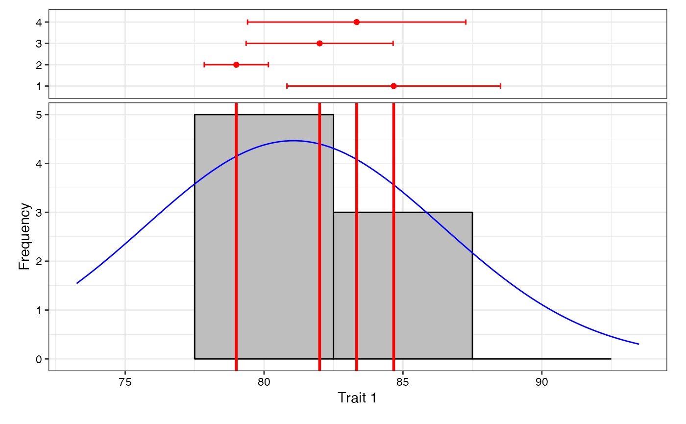
# Frequency distribution for variable y2
freq2 <- freqdist.augmentedRCBD(out2, xlab = "Trait 2")
Warning:
[1m
[22mRemoved 2 rows containing missing values or values outside the scale range
(`geom_bar()`).
plot(freq2)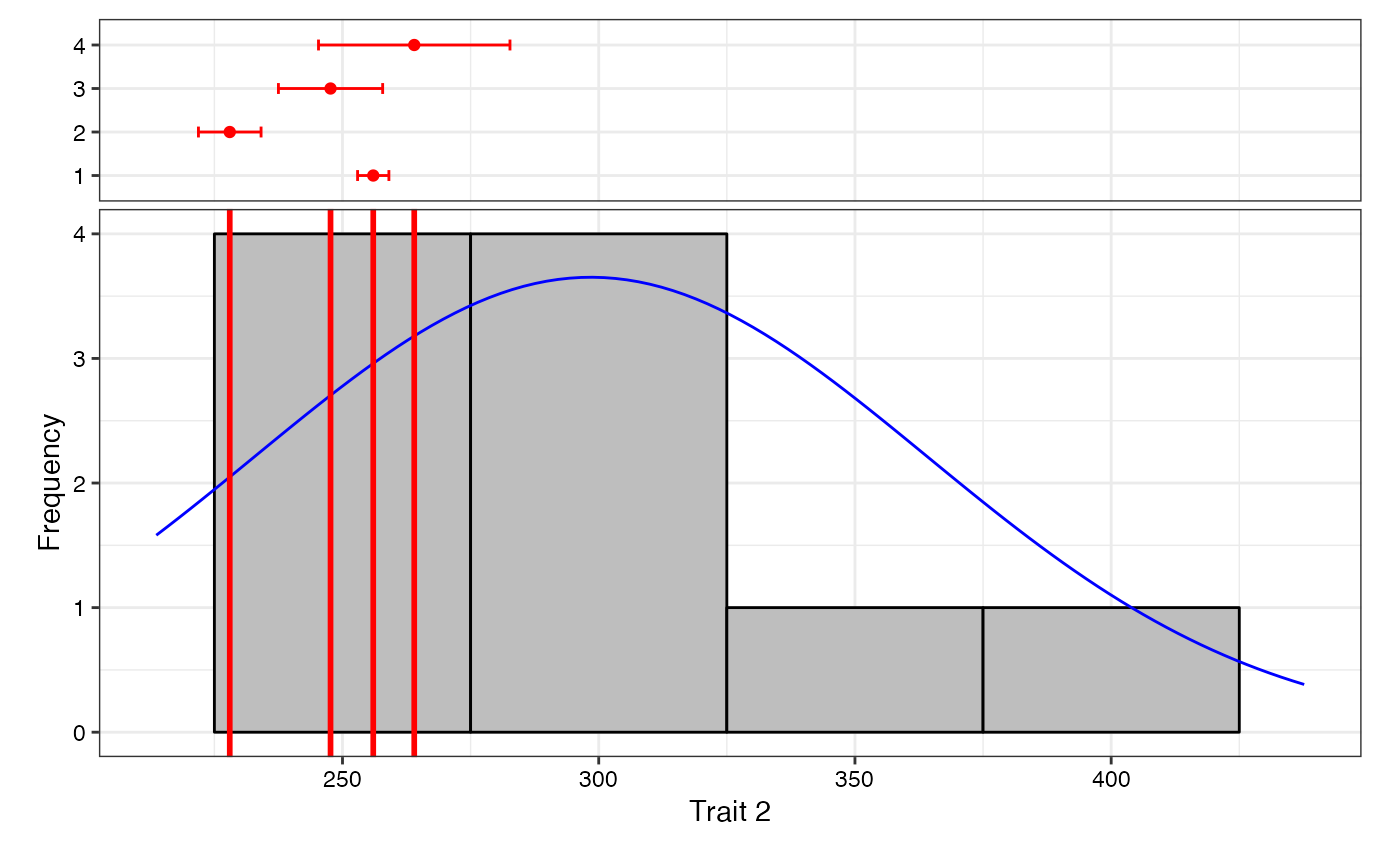
The colours for the check values may be specified using the argument
check.col.
colset <- c("red3", "green4", "purple3", "darkorange3")

# Frequency distribution for variable y1
freq1 <- freqdist.augmentedRCBD(out1, xlab = "Trait 1", check.col = colset)
Warning:
[1m
[22mRemoved 2 rows containing missing values or values outside the scale range
(`geom_bar()`).
plot(freq1)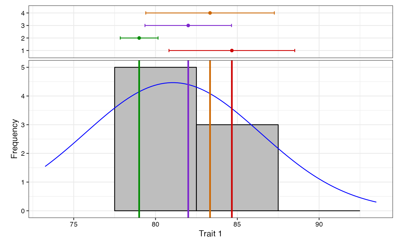
# Frequency distribution for variable y2
freq2 <- freqdist.augmentedRCBD(out2, xlab = "Trait 2", check.col = colset)
Warning:
[1m
[22mRemoved 2 rows containing missing values or values outside the scale range
(`geom_bar()`).
plot(freq2)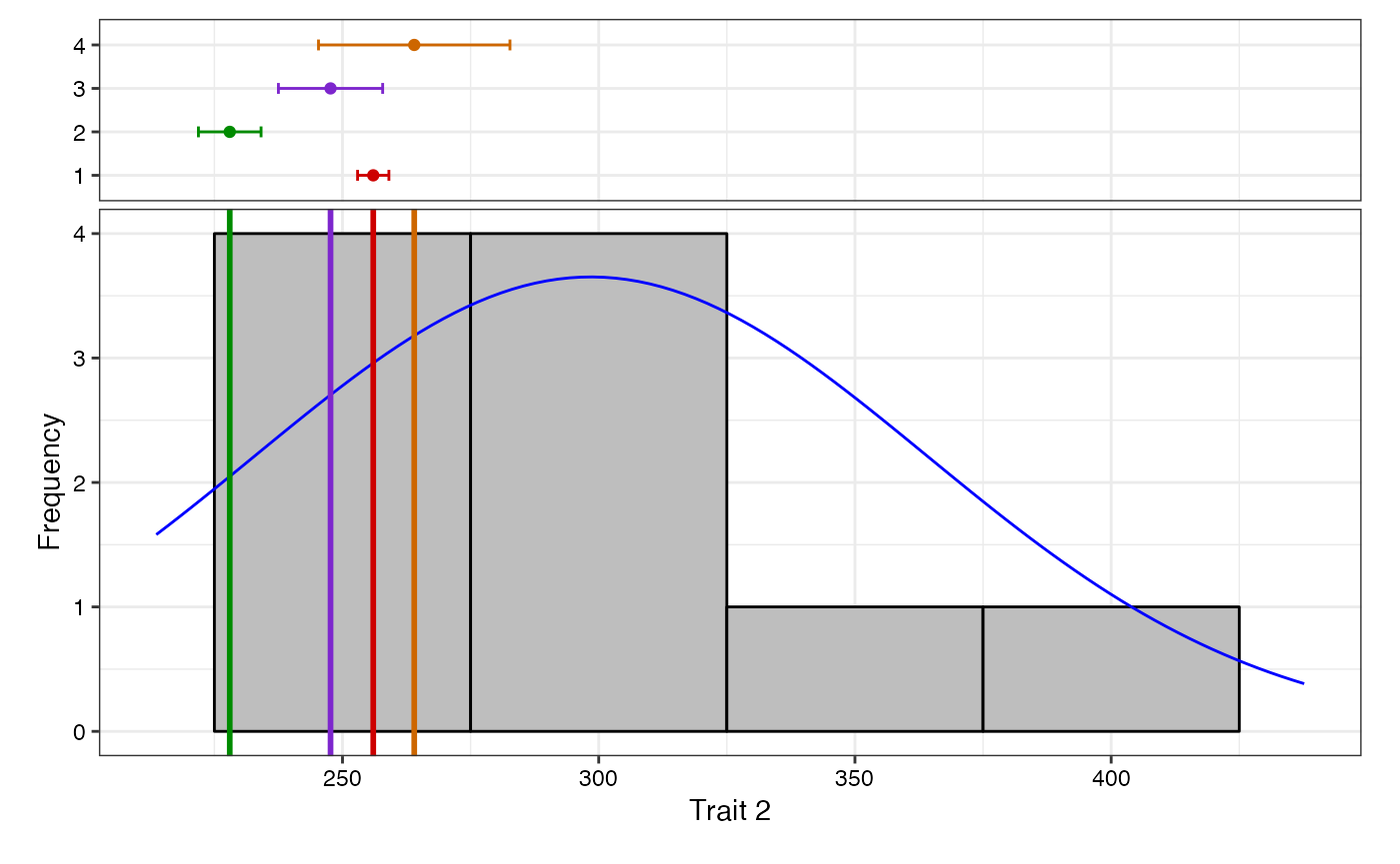
The default the check highlighting can be avoided using the argument
highlight.check = FALSE.
# Frequency distribution for variable y1
freq1 <- freqdist.augmentedRCBD(out1, xlab = "Trait 1",
                                highlight.check = FALSE)
Warning:
[1m
[22mRemoved 2 rows containing missing values or values outside the scale range
(`geom_bar()`).
plot(freq1)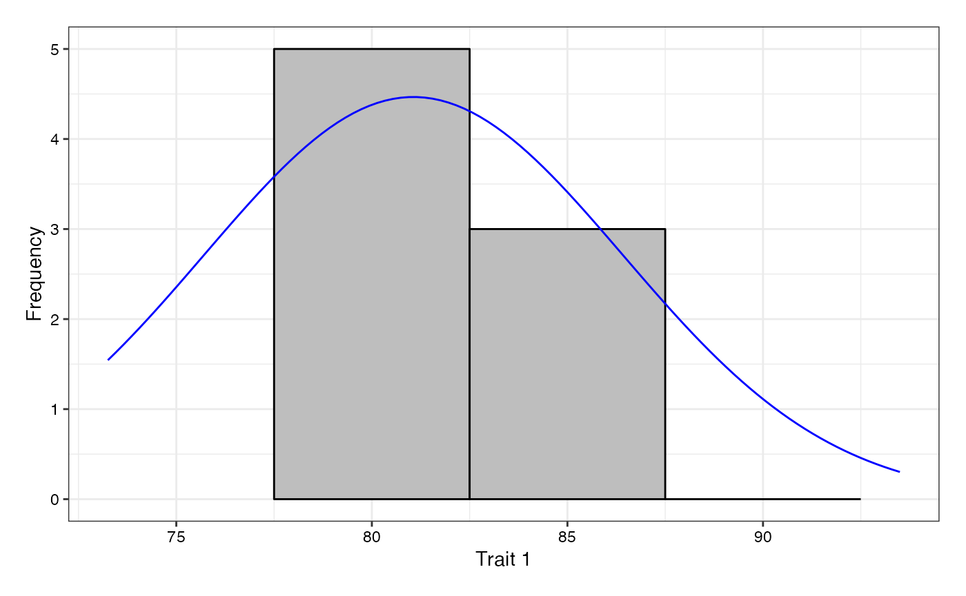
# Frequency distribution for variable y2
freq2 <- freqdist.augmentedRCBD(out2, xlab = "Trait 2",
                                highlight.check = FALSE)
Warning:
[1m
[22mRemoved 2 rows containing missing values or values outside the scale range
(`geom_bar()`).
plot(freq2)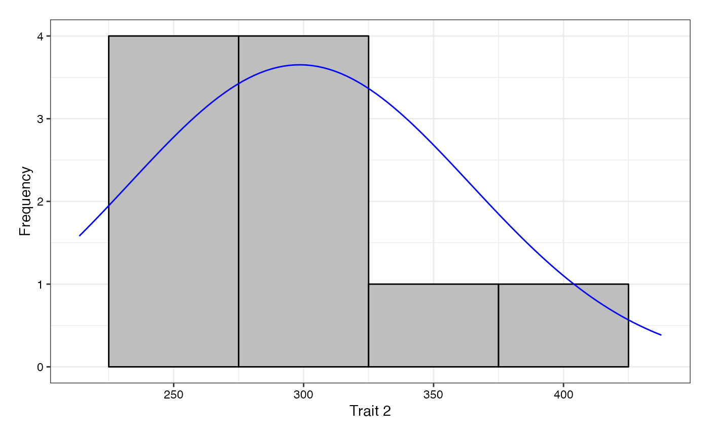
7.5 gva.augmentedRCBD()
The genetic variability statistics such as mean, phenotypic,
genotypic and environmental variation (Federer
and Searle (1976)),
phenotypic, genotypic and environmental coefficient of variation (Burton (1951), Burton (1952)), category of
phenotypic and genotypic coefficient of variation according to Sivasubramaniam and Madhavamenon (1973), broad-sense
heritability (H2) (Lush (1940)),
H2 category according to Robinson (1966), Genetic advance
(GA), genetic advance as per cent of mean (GAM) and GAM category
according to Johnson et al. (1955) are computed from an
object of class augmentedRCBD as follows. Genetic
variability analysis needs to be performed only if the sum of squares of
“Treatment: Test” are significant.
# Genetic variability statistics for variable y1
gva.augmentedRCBD(out1)
Warning in gva.augmentedRCBD(out1): P-value for "Treatment: Test" is > 0.05.
Genetic variability analysis may not be appropriate for this trait.$Mean
[1] 81.0625
$PV
[1] 72.26786
$GV
[1] 45.29563
$EV
[1] 26.97222
$GCV
[1] 8.302487
$`GCV category`
[1] "Low"
$PCV
[1] 10.48703
$`PCV category`
[1] "Medium"
$ECV
[1] 6.406759
$hBS
[1] 62.67743
$`hBS category`
[1] "High"
$GA
[1] 10.99216
$GAM
[1] 13.5601
$`GAM category`
[1] "Medium"
# Genetic variability statistics for variable y2
gva.augmentedRCBD(out2)
$Mean
[1] 298.4792
$PV
[1] 4980.411
$GV
[1] 4694.161
$EV
[1] 286.25
$GCV
[1] 22.95435
$`GCV category`
[1] "High"
$PCV
[1] 23.64387
$`PCV category`
[1] "High"
$ECV
[1] 5.668377
$hBS
[1] 94.25248
$`hBS category`
[1] "High"
$GA
[1] 137.2223
$GAM
[1] 45.97382
$`GAM category`
[1] "High"Negative estimates of variance components if computed are not abnormal. For information on how to deal with these, refer Robinson et al. (1955) and Dudley and Moll (1969).
7.5 report.augmentedRCBD()
The results generated by the analysis can be exported to a MS Word file as follows.
# MS word report for variable y1
report.augmentedRCBD(aug = out1,
                     target = file.path(tempdir(),
                                        "augmentedRCBD output.docx"),
                     file.type = "word")

# MS word report for variable y2
report.augmentedRCBD(aug = out2,
                     target = file.path(tempdir(),
                                        "augmentedRCBD output.docx"),
                     file.type = "word")
Fig. 6: MS Word report generated with
report.agumentedRCBD function.
Alternatively, the analysis results can also be exported to a MS Excel file as follows.
# MS excel report for variable y1
report.augmentedRCBD(aug = out1,
                     target = file.path(tempdir(),
                                        "augmentedRCBD output.xlsx"),
                     file.type = "excel")

# MS excel report for variable y2
report.augmentedRCBD(aug = out2,
                     target = file.path(tempdir(),
                                        "augmentedRCBD output.xlsx"),
                     file.type = "excel")
Fig. 6: MS Excel report generated with
report.agumentedRCBD function.
8 Data Analysis for a Multiple Traits
Analysis of data for a multiple traits simultaneously can be
performed by using augmentedRCBD.bulk function. It
generates an object of class augmentedRCBD.bulk. Such an
object can then be taken as input by
print.augmentedRCBD.bulk to print the results to console.
The results can also be exported as a MS Word report using the
report.augmentedRCBD.bulk function.
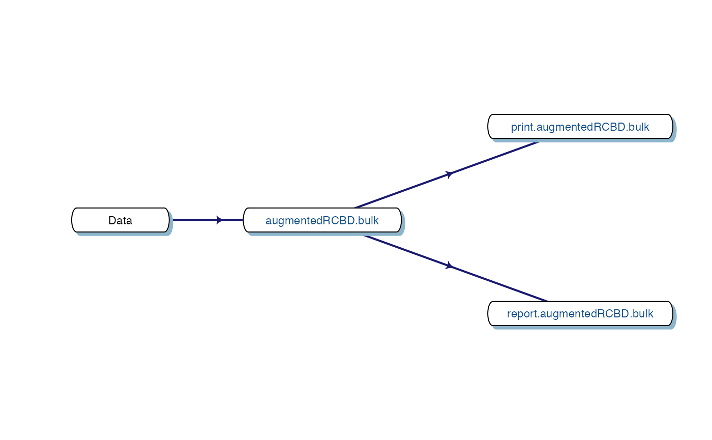
Fig. 8. Workflow for analysis of multiple traits
with augmentedRCBD.
8.1 augmentedRCBD.bulk()
Consider the data frame data imported from Table 1 according to the instructions in section 4.8.
str(data)'data.frame': 20 obs. of 4 variables:
$ blk: Factor w/ 3 levels "1","2","3": 1 1 1 1 1 1 1 2 2 2 ...
$ trt: Factor w/ 12 levels "1","2","3","4",..: 1 2 3 4 7 11 12 1 2 3 ...
$ y1 : num 92 79 87 81 96 89 82 79 81 81 ...
$ y2 : num 258 224 238 278 347 300 289 260 220 237 ...
# Convert block and treatment to factors
data$blk <- as.factor(data$blk)
data$trt <- as.factor(data$trt)
Rather than performing the analysis individually for each
variable/trait separately using augmentedRCBD, the analysis
can be performed simultaneously for for both the traits using
augmentedRCBD.bulk function. It is a wrapper around the
augmentedRCBD core function and its associated helper
functions.
However in this case treatment comparisons/grouping by least
significant difference or Tukey’s honest significant difference method
is not computed. Also the output object size is reduced using the
simplify = TRUE argument in the augmentedRCBD
function.
The logical arguments describe, freqdist
and gva can be used to specify whether to generate the
descriptive statistics, frequency distribution plots and genetic
variability statistics respectively. If gva = TRUE, then
plots to compare phenotypic and genotypic coefficient of variation,
broad sense heritability and genetic advance over mean between traits
are also generated.
bout <- augmentedRCBD.bulk(data = data, block = "blk",
                           treatment = "trt", traits = c("y1", "y2"),
                           checks = NULL, alpha = 0.05, describe = TRUE,
                           freqdist = TRUE, gva = TRUE,
                           check.col = c("brown", "darkcyan",
                                         "forestgreen", "purple"),
                           console = TRUE)
ANOVA for y1 computed (1/2)

ANOVA for y2 computed (2/2)

Augmented Design Details
========================
  Trait Number of blocks Number of treatments Number of check treatments
1    y1                3                   12                          4
2    y2                3                   12                          4
  Number of test treatments Check treatments
1                         8       1, 2, 3, 4
2                         8       1, 2, 3, 4


ANOVA, Treatment Adjusted
=========================
                                          Mean.Sq
                             Source Df     y1    Df      y2
        Block (ignoring Treatments)  2 180.04  *  2 3509.67 **
     Treatment (eliminating Blocks) 11  25.92 ⁿˢ 11 5360.49 **
                   Treatment: Check  3  17.64 ⁿˢ  3  716.75 ⁿˢ
 Treatment: Test and Test vs. Check  8  29.02 ⁿˢ  8 7101.89 **
                          Residuals  6  26.97     6  286.25
ⁿˢ P > 0.05; * P <= 0.05; ** P <= 0.01

ANOVA, Block Adjusted
=====================
                                      Mean.Sq
                         Source Df    y1    Df       y2
    Treatment (ignoring Blocks) 11 52.33 ⁿˢ 11  5882.50 **
               Treatment: Check  3 17.64 ⁿˢ  3   716.75 ⁿˢ
                Treatment: Test  7 72.27 ⁿˢ  7  4980.41 **
      Treatment: Test vs. Check  1 16.87 ⁿˢ  1 27694.41 **
 Block (eliminating Treatments)  2 34.75 ⁿˢ  2   638.58 ⁿˢ
                      Residuals  6 26.97     6   286.25
ⁿˢ P > 0.05; * P <= 0.05; ** P <= 0.01

Coefficient of Variation
========================
 Trait   CV
    y1 6.37
    y2 6.06


Overall Adjusted Mean
=====================
 Trait Overall.adjusted.mean
    y1                 81.06
    y2                298.48


Standard Errors
===============
                               Comparison   y1    y2
 A Test Treatment and a Control Treatment 6.70 21.84
                  Control Treatment Means 4.24 13.81
   Two Test Treatments (Different Blocks) 8.21 26.75
         Two Test Treatments (Same Block) 7.34 23.93


Critical Difference
===================
alpha = 0.05
                               Comparison    y1    y2
 A Test Treatment and a Control Treatment 16.41 53.45
                  Control Treatment Means 10.38 33.80
   Two Test Treatments (Different Blocks) 20.09 65.46
         Two Test Treatments (Same Block) 17.97 58.55


Descriptive Statistics
======================
 Trait Count   Mean Std.Error Std.Deviation    Min    Max Skewness Skewness_sig
    y1    12  81.06      1.55          5.36  73.25  93.50     0.93           ⁿˢ
    y2    12 298.48     18.92         65.55 213.67 437.67     0.74           ⁿˢ
 Kurtosis Kurtosis_sig
     3.52           ⁿˢ
     2.79           ⁿˢ
ⁿˢ P > 0.05; * P <= 0.05; ** P <= 0.01


Genetic Variability Analysis
============================
k = 2.063
 Trait   Mean      PV      GV     EV   GCV GCV.category   PCV PCV.category  ECV
  y1 †  81.06   72.27   45.30  26.97  8.30          Low 10.49       Medium 6.41
  y2   298.48 4980.41 4694.16 286.25 22.95         High 23.64         High 5.67
   hBS hBS.category     GA   GAM GAM.category
 62.68         High  10.99 13.56       Medium
 94.25         High 137.22 45.97         High
Warning:
† P-value for "Treatment: Test" is > 0.05. Genetic variability analysis may not be appropriate for this trait.Warning:
‡ Negative GV detected.
GCV, GCV category, hBS, hBS category,GA, GAM and
GAM category could not be computed.
Warning Messages
================


[Frequency Distribution]
<y1>
Removed 2 rows containing missing values or values outside the scale range
(`geom_bar()`).

<y2>
Removed 2 rows containing missing values or values outside the scale range
(`geom_bar()`).


[GVA]
<y1>
P-value for "Treatment: Test" is > 0.05. Genetic variability analysis may not be appropriate for this trait.


Treatment Means
===============
 Treatment Block    y1     y2
         1       84.67 256.00
        10     3 77.25 437.67
        11     1 86.50 299.42
        12     1 79.50 288.42
         2       79.00 228.00
         3       82.00 247.67
         4       83.33 264.00
         5     2 78.25 293.92
         6     3 78.25 382.67
         7     1 93.50 346.42
         8     3 73.25 213.67
         9     2 77.25 323.92
8.2 print.augmentedRCBD.bulk()
The results of analysis in an object of class
augmentedRCBD.bulk can be printed to the console as
follows.
# Print results
print(bout)
Augmented Design Details
========================
  Trait Number of blocks Number of treatments Number of check treatments
1    y1                3                   12                          4
2    y2                3                   12                          4
  Number of test treatments Check treatments
1                         8       1, 2, 3, 4
2                         8       1, 2, 3, 4


ANOVA, Treatment Adjusted
=========================
                                          Mean.Sq
                             Source Df     y1    Df      y2
        Block (ignoring Treatments)  2 180.04  *  2 3509.67 **
     Treatment (eliminating Blocks) 11  25.92 ⁿˢ 11 5360.49 **
                   Treatment: Check  3  17.64 ⁿˢ  3  716.75 ⁿˢ
 Treatment: Test and Test vs. Check  8  29.02 ⁿˢ  8 7101.89 **
                          Residuals  6  26.97     6  286.25
ⁿˢ P > 0.05; * P <= 0.05; ** P <= 0.01

ANOVA, Block Adjusted
=====================
                                      Mean.Sq
                         Source Df    y1    Df       y2
    Treatment (ignoring Blocks) 11 52.33 ⁿˢ 11  5882.50 **
               Treatment: Check  3 17.64 ⁿˢ  3   716.75 ⁿˢ
                Treatment: Test  7 72.27 ⁿˢ  7  4980.41 **
      Treatment: Test vs. Check  1 16.87 ⁿˢ  1 27694.41 **
 Block (eliminating Treatments)  2 34.75 ⁿˢ  2   638.58 ⁿˢ
                      Residuals  6 26.97     6   286.25
ⁿˢ P > 0.05; * P <= 0.05; ** P <= 0.01

Coefficient of Variation
========================
 Trait   CV
    y1 6.37
    y2 6.06


Overall Adjusted Mean
=====================
 Trait Overall.adjusted.mean
    y1                 81.06
    y2                298.48


Standard Errors
===============
                               Comparison   y1    y2
 A Test Treatment and a Control Treatment 6.70 21.84
                  Control Treatment Means 4.24 13.81
   Two Test Treatments (Different Blocks) 8.21 26.75
         Two Test Treatments (Same Block) 7.34 23.93


Critical Difference
===================
alpha = 0.05
                               Comparison    y1    y2
 A Test Treatment and a Control Treatment 16.41 53.45
                  Control Treatment Means 10.38 33.80
   Two Test Treatments (Different Blocks) 20.09 65.46
         Two Test Treatments (Same Block) 17.97 58.55


Descriptive Statistics
======================
 Trait Count   Mean Std.Error Std.Deviation    Min    Max Skewness Skewness_sig
    y1    12  81.06      1.55          5.36  73.25  93.50     0.93           ⁿˢ
    y2    12 298.48     18.92         65.55 213.67 437.67     0.74           ⁿˢ
 Kurtosis Kurtosis_sig
     3.52           ⁿˢ
     2.79           ⁿˢ
ⁿˢ P > 0.05; * P <= 0.05; ** P <= 0.01


Genetic Variability Analysis
============================
k = 2.063
 Trait   Mean      PV      GV     EV   GCV GCV.category   PCV PCV.category  ECV
  y1 †  81.06   72.27   45.30  26.97  8.30          Low 10.49       Medium 6.41
  y2   298.48 4980.41 4694.16 286.25 22.95         High 23.64         High 5.67
   hBS hBS.category     GA   GAM GAM.category
 62.68         High  10.99 13.56       Medium
 94.25         High 137.22 45.97         High
Warning:
† P-value for "Treatment: Test" is > 0.05. Genetic variability analysis may not be appropriate for this trait.Warning:
‡ Negative GV detected.
GCV, GCV category, hBS, hBS category,GA, GAM and
GAM category could not be computed.
Warning Messages
================


[Frequency Distribution]
<y1>
Removed 2 rows containing missing values or values outside the scale range
(`geom_bar()`).

<y2>
Removed 2 rows containing missing values or values outside the scale range
(`geom_bar()`).


[GVA]
<y1>
P-value for "Treatment: Test" is > 0.05. Genetic variability analysis may not be appropriate for this trait.


Treatment Means
===============
 Treatment Block    y1     y2
         1       84.67 256.00
        10     3 77.25 437.67
        11     1 86.50 299.42
        12     1 79.50 288.42
         2       79.00 228.00
         3       82.00 247.67
         4       83.33 264.00
         5     2 78.25 293.92
         6     3 78.25 382.67
         7     1 93.50 346.42
         8     3 73.25 213.67
         9     2 77.25 323.92
8.3 report.augmentedRCBD.bulk()
The results generated by the analysis can be exported to a MS Word file as follows.
# MS word report
report.augmentedRCBD.bulk(aug.bulk = bout,
                          target = file.path(tempdir(),
                                             "augmentedRCBD bulk output.docx"),
                          file.type = "word")
Fig. 9: MS Word report generated with
report.agumentedRCBD.bulk function.
Alternatively, the analysis results can also be exported to a MS Excel file as follows.
# MS excel report
report.augmentedRCBD.bulk(aug.bulk = bout,
                          target = file.path(tempdir(),
                                             "augmentedRCBD bulk output.xlsx"),
                          file.type = "excel")
Fig. 10: MS Excel report generated with
report.agumentedRCBD.bulk function.
9 Citing augmentedRCBD
To cite the R package 'augmentedRCBD' in publications use:

  Aravind, J., Mukesh Sankar, S., Wankhede, D. P., and Kaur, V. (2026).
  augmentedRCBD: Analysis of Augmented Randomised Complete Block
  Designs. R package version 0.1.7.9000,
  https://aravind-j.github.io/augmentedRCBD/https://cran.r-project.org/package=augmentedRCBD.

A BibTeX entry for LaTeX users is

  @Manual{,
    title = {augmentedRCBD: Analysis of Augmented Randomised Complete Block Designs},
    author = {J. Aravind and S. {Mukesh Sankar} and Dhammaprakash Pandhari Wankhede and Vikender Kaur},
    note = {R package version 0.1.7.9000 https://aravind-j.github.io/augmentedRCBD/ https://cran.r-project.org/package=augmentedRCBD},
    year = {2026},
  }

This free and open-source software implements academic research by the
authors and co-workers. If you use it, please support the project by
citing the package.
10 Session Info
R version 4.6.0 (2026-04-24)
Platform: aarch64-apple-darwin23
Running under: macOS Sequoia 15.7.4

Matrix products: default
BLAS:   /Library/Frameworks/R.framework/Versions/4.6/Resources/lib/libRblas.0.dylib
LAPACK: /Library/Frameworks/R.framework/Versions/4.6/Resources/lib/libRlapack.dylib;  LAPACK version 3.12.1

locale:
[1] en_US.UTF-8/en_US.UTF-8/en_US.UTF-8/C/en_US.UTF-8/en_US.UTF-8

time zone: UTC
tzcode source: internal

attached base packages:
[1] stats     graphics  grDevices utils     datasets  methods   base

other attached packages:
[1] diagram_1.6.5            shape_1.4.6.1            augmentedRCBD_0.1.7.9000

loaded via a namespace (and not attached):
 [1] tidyselect_1.2.1        dplyr_1.2.1             farver_2.1.2
 [4] bitops_1.0-9            S7_0.2.2                RCurl_1.98-1.18
 [7] fastmap_1.2.0           TH.data_1.1-5           fontquiver_0.2.1
[10] mathjaxr_2.0-0          XML_3.99-0.23           digest_0.6.39
[13] estimability_1.5.1      lifecycle_1.0.5         multcompView_0.1-11
[16] survival_3.8-6          magrittr_2.0.5          compiler_4.6.0
[19] rlang_1.2.0             sass_0.4.10             tools_4.6.0
[22] yaml_2.3.12             data.table_1.18.2.1     knitr_1.51
[25] labeling_0.4.3          askpass_1.2.1           htmlwidgets_1.6.4
[28] curl_7.1.0              plyr_1.8.9              xml2_1.5.2
[31] RColorBrewer_1.1-3      multcomp_1.4-30         numform_0.7.0
[34] withr_3.0.2             purrr_1.2.2             numDeriv_2016.8-1.1
[37] desc_1.4.3              grid_4.6.0              gdtools_0.5.0
[40] xtable_1.8-8            ggplot2_4.0.3           emmeans_2.0.3
[43] scales_1.4.0            MASS_7.3-65             cli_3.6.6
[46] mvtnorm_1.3-7           rmarkdown_2.31          ragg_1.5.2
[49] reformulas_0.4.4        generics_0.1.4          otel_0.2.0
[52] httr_1.4.8              reshape2_1.4.5          minqa_1.2.8
[55] cachem_1.1.0            stringr_1.6.0           splines_4.6.0
[58] vctrs_0.7.3             boot_1.3-32             Matrix_1.7-5
[61] sandwich_3.1-1          jsonlite_2.0.0          fontBitstreamVera_0.1.1
[64] systemfonts_1.3.2       tidyr_1.3.2             jquerylib_0.1.4
[67] glue_1.8.1              pkgdown_2.2.0.9000      nloptr_2.2.1
[70] codetools_0.2-20        stringi_1.8.7           flextable_0.9.11
[73] gtable_0.3.6            lme4_2.0-1              lmerTest_3.2-1
[76] tibble_3.3.1            pillar_1.11.1           htmltools_0.5.9
[79] openssl_2.4.0           R6_2.6.1                textshaping_1.0.5
[82] Rdpack_2.6.6            evaluate_1.0.5          lattice_0.22-9
[85] rbibutils_2.4.1         moments_0.14.1          openxlsx_4.2.8.1
[88] fontLiberation_0.1.0    bslib_0.10.0            Rcpp_1.1.1-1.1
[91] zip_2.3.3               uuid_1.2-2              nlme_3.1-169
[94] officer_0.7.4           xfun_0.57               fs_2.1.0
[97] zoo_1.8-15              pkgconfig_2.0.3