Generate Diversity Profiles for Parametric Indices
Source:R/diversity.profile.R
diversity.profile.RdGenerate Diversity Profiles for Parametric Indices
Arguments
- x
A numeric or factor vector of observations.
- group
A factor vector indicating the group of each observation. Must have the same length as
x.- q
The order of the parametric index.
- ci.conf
Confidence level of the bootstrap interval. Default is 0.95.
- R
Integer specifying the number of permutations. Default is 1000.
- parameter
The parametric index. Options include
"hill","renyi"and"tsallis". Default is"hill".- ci.type
A vector of character strings representing the type of intervals required. The options are
c("perc", "bca").- parallel
The type of parallel operation to be used (if any). If missing, the default is taken from the option
"boot.parallel"(and if that is not set,"no").- ncpus
integer: number of processes to be used in parallel operation: typically one would chose this to the number of available CPUs.
- cl
An optional parallel or snow cluster for use if
parallel = "snow". If not supplied, a cluster on the local machine is created for the duration of thebootcall.
Value
A list of data frames with the following columns for each factor
level in group.
- q
- observed
- mean
- lower
- upper
Examples
library(EvaluateCore)
library(dplyr)
#>
#> Attaching package: ‘dplyr’
#> The following objects are masked from ‘package:stats’:
#>
#> filter, lag
#> The following objects are masked from ‘package:base’:
#>
#> intersect, setdiff, setequal, union
library(ggplot2)
pdata <- cassava_CC
qual <- c("CUAL", "LNGS", "PTLC", "DSTA", "LFRT", "LBTEF", "CBTR", "NMLB",
"ANGB", "CUAL9M", "LVC9M", "TNPR9M", "PL9M", "STRP", "STRC",
"PSTR")
# Convert qualitative data columns to factor
pdata[, qual] <- lapply(pdata[, qual], as.factor)
str(pdata)
#> 'data.frame': 168 obs. of 26 variables:
#> $ CUAL : Factor w/ 4 levels "Dark green","Green purple",..: 3 1 2 2 2 2 4 2 2 1 ...
#> $ LNGS : Factor w/ 3 levels "Long","Medium",..: 3 1 2 2 2 2 2 1 1 1 ...
#> $ PTLC : Factor w/ 5 levels "Dark green","Green purple",..: 3 4 4 4 4 5 4 2 2 5 ...
#> $ DSTA : Factor w/ 5 levels "Absent","Central part",..: 1 5 5 5 5 5 5 4 2 5 ...
#> $ LFRT : Factor w/ 4 levels "25-50% leaf retention",..: 1 1 1 1 3 2 2 2 2 2 ...
#> $ LBTEF : Factor w/ 6 levels "0","1","2","3",..: 3 1 2 1 4 5 4 4 3 2 ...
#> $ CBTR : Factor w/ 3 levels "Cream","White",..: 2 2 2 2 1 2 1 1 1 1 ...
#> $ NMLB : Factor w/ 9 levels "0","1","2","3",..: 3 1 2 1 4 4 4 3 3 4 ...
#> $ ANGB : Factor w/ 4 levels "150-300","450-600",..: 1 4 1 4 2 2 2 1 2 2 ...
#> $ CUAL9M: Factor w/ 5 levels "Dark green","Green",..: 1 1 3 5 3 3 5 5 5 4 ...
#> $ LVC9M : Factor w/ 5 levels "Dark green","Green",..: 4 3 3 3 3 1 3 1 4 3 ...
#> $ TNPR9M: Factor w/ 5 levels "1","2","3","4",..: 5 5 4 2 5 4 2 5 5 5 ...
#> $ PL9M : Factor w/ 2 levels "Long (25-30cm)",..: 2 2 1 1 1 1 1 1 2 2 ...
#> $ STRP : Factor w/ 4 levels "Absent","Intermediate",..: 2 3 1 1 1 1 4 1 1 4 ...
#> $ STRC : Factor w/ 2 levels "Absent","Present": 2 2 1 2 1 1 2 1 1 2 ...
#> $ PSTR : Factor w/ 2 levels "Irregular","Tending toward horizontal": 1 2 2 2 1 2 2 2 1 2 ...
#> $ NMSR : num 6 2 6 2 20 13 4 14 10 5 ...
#> $ TTRN : num 3 0.5 3 2 5 ...
#> $ TFWSR : num 1.4 2.6 1.2 1.6 5 7 4.2 2.8 2.8 4 ...
#> $ TTRW : num 0.7 0.65 0.6 1.6 1.25 ...
#> $ TFWSS : num 1 2.8 2.8 2.4 16 12 9 4.4 6.2 5 ...
#> $ TTSW : num 0.5 0.7 1.4 2.4 4 ...
#> $ TTPW : num 2.4 5.4 4 4 21 19 13.2 7.2 9 9 ...
#> $ AVPW : num 1.2 1.35 2 4 5.25 4.75 3.3 2.4 1.8 2.25 ...
#> $ ARSR : num 2 0 2 0 3 0 0 6 0 0 ...
#> $ SRDM : num 42 39.8 29.7 43 37.9 37 38.9 36.9 41 37.9 ...
important_q <- c(0, 1, 2)
important_labels <- c("0D", "1D", "2D")
# Hill profile - Percentile CIs ----
hill_profile1 <-
diversity.profile(x = pdata$CUAL, group = pdata$LNGS,
parameter = "hill", ci.type = "perc")
hill_profile1
#> $Long
#> q observed mean lower upper
#> 1 0.0 3.000000 3.000000 3.000000 3.000000
#> 2 0.1 2.970041 2.965237 2.921973 2.992577
#> 3 0.2 2.940750 2.931635 2.849671 2.985171
#> 4 0.3 2.912153 2.899210 2.781453 2.977793
#> 5 0.4 2.884272 2.867964 2.716325 2.970595
#> 6 0.5 2.857124 2.837895 2.656209 2.963502
#> 7 0.6 2.830721 2.808990 2.602732 2.956515
#> 8 0.7 2.805073 2.781232 2.551969 2.949636
#> 9 0.8 2.780186 2.754597 2.501417 2.942864
#> 10 0.9 2.756060 2.729059 2.464737 2.936201
#> 11 1.0 2.732695 2.704587 2.427676 2.929647
#> 12 1.1 2.710085 2.681148 2.383622 2.923203
#> 13 1.2 2.688224 2.658708 2.350604 2.916868
#> 14 1.3 2.667101 2.637231 2.316516 2.910643
#> 15 1.4 2.646704 2.616681 2.282073 2.904528
#> 16 1.5 2.627019 2.597021 2.246508 2.898522
#> 17 1.6 2.608031 2.578213 2.213020 2.892625
#> 18 1.7 2.589722 2.560223 2.181418 2.886836
#> 19 1.8 2.572075 2.543013 2.162686 2.881156
#> 20 1.9 2.555070 2.526550 2.139366 2.875583
#> 21 2.0 2.538688 2.510798 2.115918 2.870115
#> 22 2.1 2.522908 2.495724 2.093917 2.863818
#> 23 2.2 2.507711 2.481296 2.073323 2.857556
#> 24 2.3 2.493075 2.467484 2.054013 2.851332
#> 25 2.4 2.478981 2.454258 2.035867 2.845149
#> 26 2.5 2.465409 2.441589 2.018802 2.839007
#> 27 2.6 2.452337 2.429449 2.002652 2.832908
#> 28 2.7 2.439748 2.417814 1.987446 2.826856
#> 29 2.8 2.427621 2.406657 1.973119 2.820851
#> 30 2.9 2.415938 2.395955 1.959608 2.814894
#> 31 3.0 2.404680 2.385687 1.946858 2.808988
#>
#> $Medium
#> q observed mean lower upper
#> 1 0.0 4.000000 3.636000 3.000000 4.000000
#> 2 0.1 3.775167 3.489633 2.923335 3.870241
#> 3 0.2 3.586424 3.361615 2.850180 3.751122
#> 4 0.3 3.427791 3.249401 2.777709 3.644197
#> 5 0.4 3.293906 3.150653 2.711803 3.544808
#> 6 0.5 3.180150 3.063299 2.645455 3.456135
#> 7 0.6 3.082659 2.985560 2.581794 3.379397
#> 8 0.7 2.998274 2.915938 2.520959 3.318026
#> 9 0.8 2.924454 2.853186 2.463044 3.254422
#> 10 0.9 2.859178 2.796281 2.408107 3.203313
#> 11 1.0 2.800853 2.744383 2.334279 3.155736
#> 12 1.1 2.748230 2.696806 2.282210 3.121258
#> 13 1.2 2.700330 2.652989 2.233528 3.075917
#> 14 1.3 2.656390 2.612469 2.182945 3.035122
#> 15 1.4 2.615811 2.574865 2.133718 3.001715
#> 16 1.5 2.578125 2.539861 2.092109 2.961438
#> 17 1.6 2.542961 2.507191 2.056051 2.928476
#> 18 1.7 2.510025 2.476629 2.022449 2.903911
#> 19 1.8 2.479080 2.447983 1.991352 2.880936
#> 20 1.9 2.449934 2.421089 1.962551 2.859325
#> 21 2.0 2.422430 2.395800 1.935809 2.842027
#> 22 2.1 2.396434 2.371990 1.911049 2.833887
#> 23 2.2 2.371835 2.349546 1.888168 2.823094
#> 24 2.3 2.348536 2.328368 1.867017 2.812977
#> 25 2.4 2.326451 2.308365 1.847333 2.795175
#> 26 2.5 2.305505 2.289455 1.829078 2.778113
#> 27 2.6 2.285629 2.271564 1.812137 2.771329
#> 28 2.7 2.266761 2.254623 1.796402 2.764668
#> 29 2.8 2.248843 2.238569 1.781771 2.757032
#> 30 2.9 2.231821 2.223347 1.768160 2.744732
#> 31 3.0 2.215647 2.208901 1.755484 2.730109
#>
#> $Short
#> q observed mean lower upper
#> 1 0.0 4.000000 3.896000 3.000000 4.000000
#> 2 0.1 3.933810 3.811891 2.945488 3.985467
#> 3 0.2 3.870196 3.732724 2.892852 3.971064
#> 4 0.3 3.809136 3.658363 2.842166 3.956734
#> 5 0.4 3.750595 3.588635 2.793517 3.941970
#> 6 0.5 3.694521 3.523332 2.746901 3.927051
#> 7 0.6 3.640856 3.462230 2.702322 3.911985
#> 8 0.7 3.589527 3.405091 2.642540 3.896783
#> 9 0.8 3.540459 3.351672 2.595904 3.881456
#> 10 0.9 3.493567 3.301732 2.544475 3.866015
#> 11 1.0 3.448767 3.255034 2.477550 3.850473
#> 12 1.1 3.405970 3.211352 2.408771 3.834840
#> 13 1.2 3.365087 3.170467 2.363287 3.819131
#> 14 1.3 3.326031 3.132176 2.328314 3.803358
#> 15 1.4 3.288713 3.096286 2.268437 3.787535
#> 16 1.5 3.253050 3.062619 2.214538 3.771675
#> 17 1.6 3.218958 3.031008 2.165962 3.755792
#> 18 1.7 3.186359 3.001300 2.122119 3.739900
#> 19 1.8 3.155176 2.973354 2.082796 3.724012
#> 20 1.9 3.125338 2.947038 2.047367 3.708144
#> 21 2.0 3.096774 2.922233 2.014700 3.692308
#> 22 2.1 3.069420 2.898829 1.984990 3.683045
#> 23 2.2 3.043214 2.876724 1.957911 3.674198
#> 24 2.3 3.018098 2.855824 1.933178 3.665745
#> 25 2.4 2.994016 2.836046 1.910541 3.657669
#> 26 2.5 2.970917 2.817309 1.889778 3.649951
#> 27 2.6 2.948751 2.799542 1.870694 3.642573
#> 28 2.7 2.927474 2.782679 1.853118 3.635520
#> 29 2.8 2.907041 2.766659 1.836899 3.628774
#> 30 2.9 2.887412 2.751424 1.821903 3.622398
#> 31 3.0 2.868549 2.736925 1.808011 3.616389
#>
#> attr(,"R")
#> [1] 1000
#> attr(,"conf")
#> [1] 0.95
#> attr(,"parameter")
#> [1] "hill"
#> attr(,"ci.type")
#> [1] "perc"
hill_profile1_df <- dplyr::bind_rows(hill_profile1, .id = "group")
hill_points1_df <- hill_profile1_df %>%
filter(q %in% important_q) %>%
mutate(order_label = factor(q, levels = important_q,
labels = important_labels))
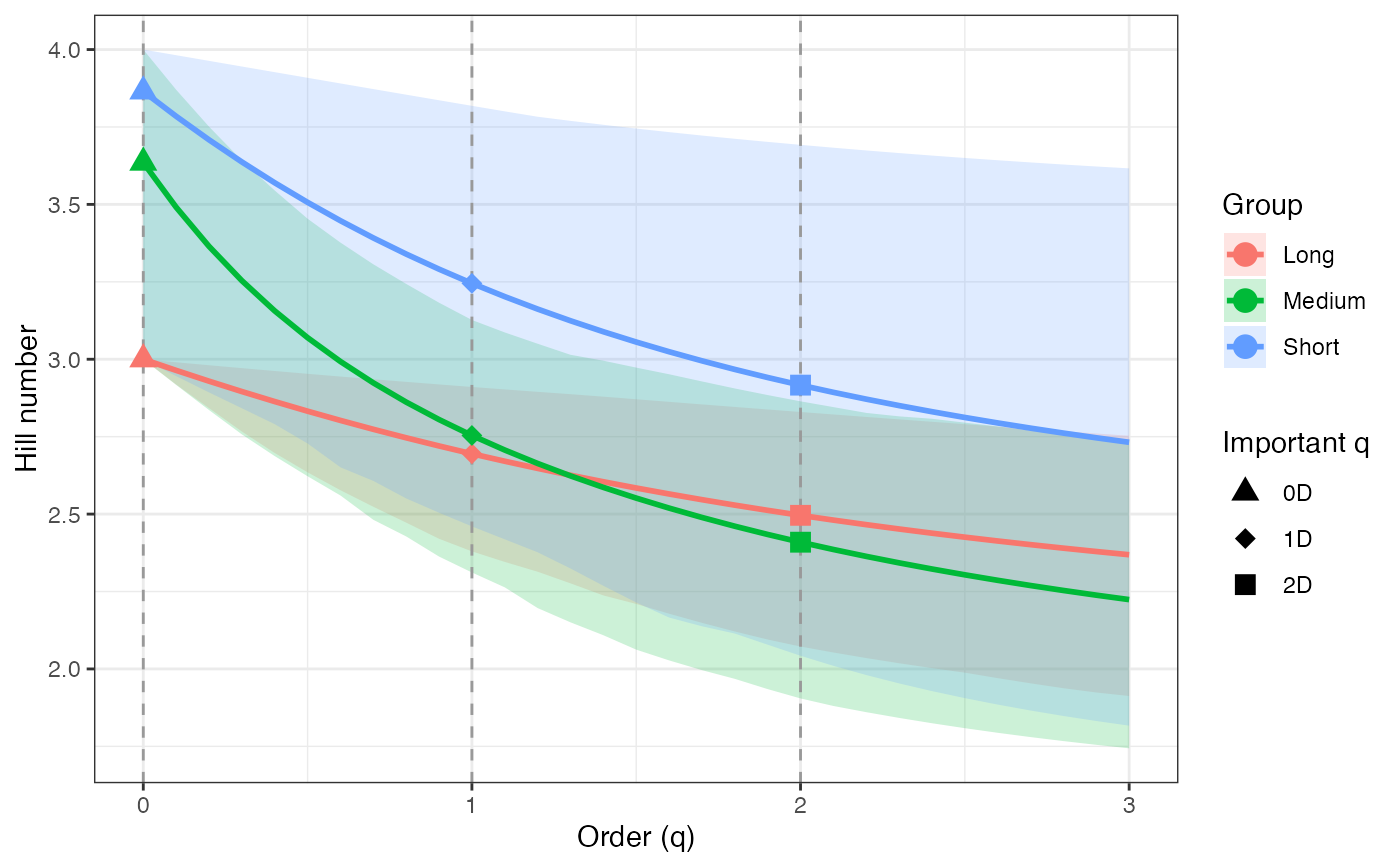
ggplot(hill_profile1_df, aes(x = q, y = mean,
color = group, fill = group)) +
geom_ribbon(aes(ymin = lower, ymax = upper), alpha = 0.2, color = NA) +
geom_line(linewidth = 1) +
geom_vline(xintercept = c(0, 1, 2), linetype = "dashed",
color = "grey60") +
geom_point(data = hill_points1_df, aes(shape = order_label),
size = 3, stroke = 1, inherit.aes = TRUE) +
scale_shape_manual(values = c(17, 18, 15), name = "Important q") +
labs(x = "Order (q)", y = "Hill number",
color = "Group", fill = "Group") +
theme_bw()
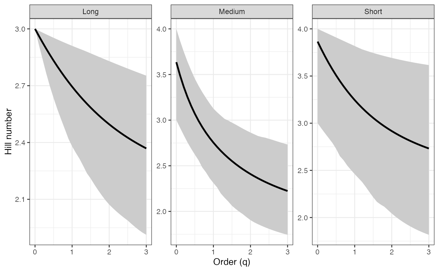
 ggplot(hill_profile1_df, aes(x = q, y = mean)) +
geom_ribbon(aes(ymin = lower, ymax = upper), fill = "grey80") +
geom_line(color = "black", linewidth = 1) +
facet_wrap(~ group, scales = "free_y") +
labs(x = "Order (q)", y = "Hill number") +
theme_bw()
ggplot(hill_profile1_df, aes(x = q, y = mean)) +
geom_ribbon(aes(ymin = lower, ymax = upper), fill = "grey80") +
geom_line(color = "black", linewidth = 1) +
facet_wrap(~ group, scales = "free_y") +
labs(x = "Order (q)", y = "Hill number") +
theme_bw()
 # Rényi profile - Percentile CIs ----
renyi_profile1 <-
diversity.profile(pdata$CUAL, group = pdata$LNGS,
parameter = "renyi", ci.type = "perc")
renyi_profile1
#> $Long
#> q observed mean lower upper
#> 1 0.0 1.0986123 1.0986123 1.0986123 1.098612
#> 2 0.1 1.0885756 1.0869593 1.0735580 1.096135
#> 3 0.2 1.0786646 1.0755145 1.0499397 1.093657
#> 4 0.3 1.0688928 1.0642985 1.0263699 1.091182
#> 5 0.4 1.0592726 1.0533291 1.0031111 1.088764
#> 6 0.5 1.0498155 1.0426209 0.9803949 1.086375
#> 7 0.6 1.0405315 1.0321858 0.9582883 1.084018
#> 8 0.7 1.0314297 1.0220329 0.9375251 1.081692
#> 9 0.8 1.0225177 1.0121689 0.9197417 1.079397
#> 10 0.9 1.0138021 1.0025981 0.9031533 1.077135
#> 11 1.0 1.0052882 0.9933228 0.8838802 1.074906
#> 12 1.1 0.9969801 0.9843435 0.8643204 1.072710
#> 13 1.2 0.9888807 0.9756588 0.8499650 1.070547
#> 14 1.3 0.9809920 0.9672663 0.8340407 1.068418
#> 15 1.4 0.9733151 0.9591621 0.8178788 1.066323
#> 16 1.5 0.9658499 0.9513412 0.8088280 1.064261
#> 17 1.6 0.9585956 0.9437980 0.7942839 1.062234
#> 18 1.7 0.9515507 0.9365260 0.7798622 1.060240
#> 19 1.8 0.9447130 0.9295183 0.7661068 1.058280
#> 20 1.9 0.9380796 0.9227673 0.7530072 1.056355
#> 21 2.0 0.9316472 0.9162654 0.7405494 1.054463
#> 22 2.1 0.9254122 0.9100045 0.7287438 1.052604
#> 23 2.2 0.9193702 0.9039764 0.7175603 1.050779
#> 24 2.3 0.9135169 0.8981731 0.7069563 1.048987
#> 25 2.4 0.9078477 0.8925863 0.6968700 1.047228
#> 26 2.5 0.9023576 0.8872078 0.6873032 1.045501
#> 27 2.6 0.8970416 0.8820296 0.6782448 1.043807
#> 28 2.7 0.8918947 0.8770438 0.6696699 1.042145
#> 29 2.8 0.8869118 0.8722427 0.6615533 1.040515
#> 30 2.9 0.8820876 0.8676187 0.6538708 1.038916
#> 31 3.0 0.8774170 0.8631645 0.6465983 1.037347
#>
#> $Medium
#> q observed mean lower upper
#> 1 0.0 1.3862944 1.2847426 1.0986123 1.386294
#> 2 0.1 1.3284446 1.2453194 1.0726418 1.353458
#> 3 0.2 1.2771555 1.2090842 1.0464656 1.322471
#> 4 0.3 1.2319160 1.1758793 1.0202116 1.293143
#> 5 0.4 1.1920742 1.1454745 0.9948555 1.266112
#> 6 0.5 1.1569284 1.1176048 0.9698758 1.241912
#> 7 0.6 1.1257925 1.0919986 0.9443960 1.220564
#> 8 0.7 1.0980367 1.0683967 0.9193111 1.200033
#> 9 0.8 1.0731077 1.0465629 0.8947414 1.181778
#> 10 0.9 1.0505342 1.0262883 0.8705714 1.161900
#> 11 1.0 1.0299241 1.0073925 0.8452074 1.148927
#> 12 1.1 1.0109570 0.9897214 0.8227730 1.134204
#> 13 1.2 0.9933740 0.9731445 0.8012190 1.121715
#> 14 1.3 0.9769680 0.9575520 0.7779993 1.111116
#> 15 1.4 0.9615743 0.9428509 0.7533364 1.101719
#> 16 1.5 0.9470625 0.9289627 0.7321059 1.091446
#> 17 1.6 0.9333293 0.9158203 0.7150167 1.083735
#> 18 1.7 0.9202928 0.9033663 0.6989213 1.075516
#> 19 1.8 0.9078876 0.8915508 0.6837638 1.067745
#> 20 1.9 0.8960613 0.8803300 0.6695241 1.058965
#> 21 2.0 0.8847711 0.8696653 0.6561662 1.052250
#> 22 2.1 0.8739819 0.8595220 0.6459005 1.047848
#> 23 2.2 0.8636641 0.8498688 0.6363017 1.043664
#> 24 2.3 0.8537922 0.8406773 0.6265899 1.039355
#> 25 2.4 0.8443440 0.8319212 0.6157903 1.034079
#> 26 2.5 0.8352998 0.8235763 0.6056715 1.027598
#> 27 2.6 0.8266413 0.8156201 0.5961912 1.021302
#> 28 2.7 0.8183519 0.8080316 0.5873087 1.015433
#> 29 2.8 0.8104158 0.8007910 0.5788767 1.011993
#> 30 2.9 0.8028180 0.7938798 0.5709934 1.009272
#> 31 3.0 0.7955444 0.7872807 0.5636211 1.006602
#>
#> $Short
#> q observed mean lower upper
#> 1 0.0 1.386294 1.3506218 1.0986123 1.386294
#> 2 0.1 1.369609 1.3297027 1.0802640 1.382655
#> 3 0.2 1.353305 1.3094178 1.0622339 1.379034
#> 4 0.3 1.337402 1.2898111 1.0443952 1.375435
#> 5 0.4 1.321914 1.2709141 1.0261438 1.371860
#> 6 0.5 1.306851 1.2527474 1.0079079 1.368309
#> 7 0.6 1.292219 1.2353211 0.9897522 1.364787
#> 8 0.7 1.278021 1.2186367 0.9717405 1.361293
#> 9 0.8 1.264256 1.2026882 0.9539348 1.357829
#> 10 0.9 1.250923 1.1874634 0.9229697 1.354398
#> 11 1.0 1.238017 1.1729453 0.9004243 1.351001
#> 12 1.1 1.225530 1.1591130 0.8831375 1.347639
#> 13 1.2 1.213454 1.1459427 0.8656782 1.344313
#> 14 1.3 1.201780 1.1334089 0.8451444 1.341026
#> 15 1.4 1.190496 1.1214846 0.8190911 1.337777
#> 16 1.5 1.179593 1.1101422 0.7950438 1.334568
#> 17 1.6 1.169058 1.0993539 0.7728647 1.331401
#> 18 1.7 1.158879 1.0890921 0.7597670 1.328275
#> 19 1.8 1.149044 1.0793297 0.7487014 1.325191
#> 20 1.9 1.139542 1.0700404 0.7315397 1.322151
#> 21 2.0 1.130361 1.0611986 0.7142006 1.319155
#> 22 2.1 1.121489 1.0527799 0.6981423 1.316203
#> 23 2.2 1.112914 1.0447607 0.6832689 1.313296
#> 24 2.3 1.104627 1.0371189 0.6694889 1.310434
#> 25 2.4 1.096616 1.0298332 0.6567161 1.307617
#> 26 2.5 1.088871 1.0228835 0.6448696 1.304846
#> 27 2.6 1.081382 1.0162509 0.6338744 1.302121
#> 28 2.7 1.074140 1.0099175 0.6236607 1.299441
#> 29 2.8 1.067136 1.0038664 0.6141642 1.296806
#> 30 2.9 1.060361 0.9980818 0.6053259 1.294217
#> 31 3.0 1.053806 0.9925487 0.5970915 1.291673
#>
#> attr(,"R")
#> [1] 1000
#> attr(,"conf")
#> [1] 0.95
#> attr(,"parameter")
#> [1] "renyi"
#> attr(,"ci.type")
#> [1] "perc"
renyi_profile1_df <- dplyr::bind_rows(renyi_profile1, .id = "group")
renyi_points1_df <- renyi_profile1_df %>%
filter(q %in% important_q) %>%
mutate(order_label = factor(q, levels = important_q,
labels = important_labels))
ggplot(renyi_profile1_df, aes(x = q, y = mean,
color = group, fill = group)) +
geom_ribbon(aes(ymin = lower, ymax = upper), alpha = 0.2, color = NA) +
geom_line(linewidth = 1) +
geom_vline(xintercept = c(0, 1, 2), linetype = "dashed",
color = "grey60") +
geom_point(data = renyi_points1_df, aes(shape = order_label),
size = 3, stroke = 1, inherit.aes = TRUE) +
scale_shape_manual(values = c(17, 18, 15), name = "Important q") +
labs(x = "Order (q)", y = "Hill number",
color = "Group", fill = "Group") +
theme_bw()
# Rényi profile - Percentile CIs ----
renyi_profile1 <-
diversity.profile(pdata$CUAL, group = pdata$LNGS,
parameter = "renyi", ci.type = "perc")
renyi_profile1
#> $Long
#> q observed mean lower upper
#> 1 0.0 1.0986123 1.0986123 1.0986123 1.098612
#> 2 0.1 1.0885756 1.0869593 1.0735580 1.096135
#> 3 0.2 1.0786646 1.0755145 1.0499397 1.093657
#> 4 0.3 1.0688928 1.0642985 1.0263699 1.091182
#> 5 0.4 1.0592726 1.0533291 1.0031111 1.088764
#> 6 0.5 1.0498155 1.0426209 0.9803949 1.086375
#> 7 0.6 1.0405315 1.0321858 0.9582883 1.084018
#> 8 0.7 1.0314297 1.0220329 0.9375251 1.081692
#> 9 0.8 1.0225177 1.0121689 0.9197417 1.079397
#> 10 0.9 1.0138021 1.0025981 0.9031533 1.077135
#> 11 1.0 1.0052882 0.9933228 0.8838802 1.074906
#> 12 1.1 0.9969801 0.9843435 0.8643204 1.072710
#> 13 1.2 0.9888807 0.9756588 0.8499650 1.070547
#> 14 1.3 0.9809920 0.9672663 0.8340407 1.068418
#> 15 1.4 0.9733151 0.9591621 0.8178788 1.066323
#> 16 1.5 0.9658499 0.9513412 0.8088280 1.064261
#> 17 1.6 0.9585956 0.9437980 0.7942839 1.062234
#> 18 1.7 0.9515507 0.9365260 0.7798622 1.060240
#> 19 1.8 0.9447130 0.9295183 0.7661068 1.058280
#> 20 1.9 0.9380796 0.9227673 0.7530072 1.056355
#> 21 2.0 0.9316472 0.9162654 0.7405494 1.054463
#> 22 2.1 0.9254122 0.9100045 0.7287438 1.052604
#> 23 2.2 0.9193702 0.9039764 0.7175603 1.050779
#> 24 2.3 0.9135169 0.8981731 0.7069563 1.048987
#> 25 2.4 0.9078477 0.8925863 0.6968700 1.047228
#> 26 2.5 0.9023576 0.8872078 0.6873032 1.045501
#> 27 2.6 0.8970416 0.8820296 0.6782448 1.043807
#> 28 2.7 0.8918947 0.8770438 0.6696699 1.042145
#> 29 2.8 0.8869118 0.8722427 0.6615533 1.040515
#> 30 2.9 0.8820876 0.8676187 0.6538708 1.038916
#> 31 3.0 0.8774170 0.8631645 0.6465983 1.037347
#>
#> $Medium
#> q observed mean lower upper
#> 1 0.0 1.3862944 1.2847426 1.0986123 1.386294
#> 2 0.1 1.3284446 1.2453194 1.0726418 1.353458
#> 3 0.2 1.2771555 1.2090842 1.0464656 1.322471
#> 4 0.3 1.2319160 1.1758793 1.0202116 1.293143
#> 5 0.4 1.1920742 1.1454745 0.9948555 1.266112
#> 6 0.5 1.1569284 1.1176048 0.9698758 1.241912
#> 7 0.6 1.1257925 1.0919986 0.9443960 1.220564
#> 8 0.7 1.0980367 1.0683967 0.9193111 1.200033
#> 9 0.8 1.0731077 1.0465629 0.8947414 1.181778
#> 10 0.9 1.0505342 1.0262883 0.8705714 1.161900
#> 11 1.0 1.0299241 1.0073925 0.8452074 1.148927
#> 12 1.1 1.0109570 0.9897214 0.8227730 1.134204
#> 13 1.2 0.9933740 0.9731445 0.8012190 1.121715
#> 14 1.3 0.9769680 0.9575520 0.7779993 1.111116
#> 15 1.4 0.9615743 0.9428509 0.7533364 1.101719
#> 16 1.5 0.9470625 0.9289627 0.7321059 1.091446
#> 17 1.6 0.9333293 0.9158203 0.7150167 1.083735
#> 18 1.7 0.9202928 0.9033663 0.6989213 1.075516
#> 19 1.8 0.9078876 0.8915508 0.6837638 1.067745
#> 20 1.9 0.8960613 0.8803300 0.6695241 1.058965
#> 21 2.0 0.8847711 0.8696653 0.6561662 1.052250
#> 22 2.1 0.8739819 0.8595220 0.6459005 1.047848
#> 23 2.2 0.8636641 0.8498688 0.6363017 1.043664
#> 24 2.3 0.8537922 0.8406773 0.6265899 1.039355
#> 25 2.4 0.8443440 0.8319212 0.6157903 1.034079
#> 26 2.5 0.8352998 0.8235763 0.6056715 1.027598
#> 27 2.6 0.8266413 0.8156201 0.5961912 1.021302
#> 28 2.7 0.8183519 0.8080316 0.5873087 1.015433
#> 29 2.8 0.8104158 0.8007910 0.5788767 1.011993
#> 30 2.9 0.8028180 0.7938798 0.5709934 1.009272
#> 31 3.0 0.7955444 0.7872807 0.5636211 1.006602
#>
#> $Short
#> q observed mean lower upper
#> 1 0.0 1.386294 1.3506218 1.0986123 1.386294
#> 2 0.1 1.369609 1.3297027 1.0802640 1.382655
#> 3 0.2 1.353305 1.3094178 1.0622339 1.379034
#> 4 0.3 1.337402 1.2898111 1.0443952 1.375435
#> 5 0.4 1.321914 1.2709141 1.0261438 1.371860
#> 6 0.5 1.306851 1.2527474 1.0079079 1.368309
#> 7 0.6 1.292219 1.2353211 0.9897522 1.364787
#> 8 0.7 1.278021 1.2186367 0.9717405 1.361293
#> 9 0.8 1.264256 1.2026882 0.9539348 1.357829
#> 10 0.9 1.250923 1.1874634 0.9229697 1.354398
#> 11 1.0 1.238017 1.1729453 0.9004243 1.351001
#> 12 1.1 1.225530 1.1591130 0.8831375 1.347639
#> 13 1.2 1.213454 1.1459427 0.8656782 1.344313
#> 14 1.3 1.201780 1.1334089 0.8451444 1.341026
#> 15 1.4 1.190496 1.1214846 0.8190911 1.337777
#> 16 1.5 1.179593 1.1101422 0.7950438 1.334568
#> 17 1.6 1.169058 1.0993539 0.7728647 1.331401
#> 18 1.7 1.158879 1.0890921 0.7597670 1.328275
#> 19 1.8 1.149044 1.0793297 0.7487014 1.325191
#> 20 1.9 1.139542 1.0700404 0.7315397 1.322151
#> 21 2.0 1.130361 1.0611986 0.7142006 1.319155
#> 22 2.1 1.121489 1.0527799 0.6981423 1.316203
#> 23 2.2 1.112914 1.0447607 0.6832689 1.313296
#> 24 2.3 1.104627 1.0371189 0.6694889 1.310434
#> 25 2.4 1.096616 1.0298332 0.6567161 1.307617
#> 26 2.5 1.088871 1.0228835 0.6448696 1.304846
#> 27 2.6 1.081382 1.0162509 0.6338744 1.302121
#> 28 2.7 1.074140 1.0099175 0.6236607 1.299441
#> 29 2.8 1.067136 1.0038664 0.6141642 1.296806
#> 30 2.9 1.060361 0.9980818 0.6053259 1.294217
#> 31 3.0 1.053806 0.9925487 0.5970915 1.291673
#>
#> attr(,"R")
#> [1] 1000
#> attr(,"conf")
#> [1] 0.95
#> attr(,"parameter")
#> [1] "renyi"
#> attr(,"ci.type")
#> [1] "perc"
renyi_profile1_df <- dplyr::bind_rows(renyi_profile1, .id = "group")
renyi_points1_df <- renyi_profile1_df %>%
filter(q %in% important_q) %>%
mutate(order_label = factor(q, levels = important_q,
labels = important_labels))
ggplot(renyi_profile1_df, aes(x = q, y = mean,
color = group, fill = group)) +
geom_ribbon(aes(ymin = lower, ymax = upper), alpha = 0.2, color = NA) +
geom_line(linewidth = 1) +
geom_vline(xintercept = c(0, 1, 2), linetype = "dashed",
color = "grey60") +
geom_point(data = renyi_points1_df, aes(shape = order_label),
size = 3, stroke = 1, inherit.aes = TRUE) +
scale_shape_manual(values = c(17, 18, 15), name = "Important q") +
labs(x = "Order (q)", y = "Hill number",
color = "Group", fill = "Group") +
theme_bw()
 ggplot(renyi_profile1_df, aes(x = q, y = mean)) +
geom_ribbon(aes(ymin = lower, ymax = upper), fill = "grey80") +
geom_line(color = "black", linewidth = 1) +
facet_wrap(~ group, scales = "free_y") +
labs(x = "Order (q)", y = "Hill number") +
theme_bw()
ggplot(renyi_profile1_df, aes(x = q, y = mean)) +
geom_ribbon(aes(ymin = lower, ymax = upper), fill = "grey80") +
geom_line(color = "black", linewidth = 1) +
facet_wrap(~ group, scales = "free_y") +
labs(x = "Order (q)", y = "Hill number") +
theme_bw()
 # Tsallis profile - Percentile CIs ----
tsallis_profile1 <-
diversity.profile(pdata$CUAL, group = pdata$LNGS,
parameter = "tsallis", ci.type = "perc")
tsallis_profile1 <-
diversity.profile(x = pdata$CUAL, group = pdata$LNGS,
parameter = "hill", ci.type = "perc")
tsallis_profile1
#> $Long
#> q observed mean lower upper
#> 1 0.0 3.000000 3.000000 3.000000 3.000000
#> 2 0.1 2.970041 2.964772 2.920375 2.991956
#> 3 0.2 2.940750 2.930709 2.846249 2.984001
#> 4 0.3 2.912153 2.897824 2.777695 2.976009
#> 5 0.4 2.884272 2.866124 2.711803 2.967954
#> 6 0.5 2.857124 2.835605 2.645470 2.959878
#> 7 0.6 2.830721 2.806255 2.581904 2.951784
#> 8 0.7 2.805073 2.778059 2.526575 2.943676
#> 9 0.8 2.780186 2.750993 2.483356 2.935559
#> 10 0.9 2.756060 2.725033 2.432103 2.927437
#> 11 1.0 2.732695 2.700148 2.395739 2.919314
#> 12 1.1 2.710085 2.676305 2.359741 2.911195
#> 13 1.2 2.688224 2.653472 2.318636 2.903083
#> 14 1.3 2.667101 2.631612 2.281339 2.894984
#> 15 1.4 2.646704 2.610690 2.251086 2.886902
#> 16 1.5 2.627019 2.590669 2.223113 2.878840
#> 17 1.6 2.608031 2.571512 2.197246 2.870804
#> 18 1.7 2.589722 2.553183 2.166901 2.862797
#> 19 1.8 2.572075 2.535647 2.141263 2.854823
#> 20 1.9 2.555070 2.518867 2.117589 2.848274
#> 21 2.0 2.538688 2.502810 2.095434 2.842027
#> 22 2.1 2.522908 2.487443 2.074753 2.834278
#> 23 2.2 2.507711 2.472732 2.055434 2.826724
#> 24 2.3 2.493075 2.458648 2.037277 2.820827
#> 25 2.4 2.478981 2.445161 2.018504 2.815084
#> 26 2.5 2.465409 2.432240 1.998596 2.809492
#> 27 2.6 2.452337 2.419860 1.979917 2.804047
#> 28 2.7 2.439748 2.407993 1.962391 2.798747
#> 29 2.8 2.427621 2.396616 1.949113 2.793588
#> 30 2.9 2.415938 2.385702 1.937464 2.788567
#> 31 3.0 2.404680 2.375231 1.926447 2.783681
#>
#> $Medium
#> q observed mean lower upper
#> 1 0.0 4.000000 3.629000 3.000000 4.000000
#> 2 0.1 3.775167 3.485460 2.924505 3.876119
#> 3 0.2 3.586424 3.359704 2.850187 3.763158
#> 4 0.3 3.427791 3.249286 2.777431 3.660512
#> 5 0.4 3.293906 3.151957 2.706542 3.566668
#> 6 0.5 3.180150 3.065724 2.645455 3.481459
#> 7 0.6 3.082659 2.988874 2.581794 3.403982
#> 8 0.7 2.998274 2.919958 2.520959 3.324892
#> 9 0.8 2.924454 2.857774 2.455032 3.264034
#> 10 0.9 2.859178 2.801326 2.392274 3.194809
#> 11 1.0 2.800853 2.749801 2.336744 3.152596
#> 12 1.1 2.748230 2.702530 2.288113 3.101517
#> 13 1.2 2.700330 2.658963 2.242776 3.055269
#> 14 1.3 2.656390 2.618651 2.188194 3.015622
#> 15 1.4 2.615811 2.581218 2.145190 2.990795
#> 16 1.5 2.578125 2.546354 2.105357 2.955542
#> 17 1.6 2.542961 2.513798 2.068318 2.922787
#> 18 1.7 2.510025 2.483327 2.033782 2.906173
#> 19 1.8 2.479080 2.454754 2.001963 2.882575
#> 20 1.9 2.449934 2.427915 1.972356 2.863877
#> 21 2.0 2.422430 2.402667 1.944743 2.851407
#> 22 2.1 2.396434 2.378884 1.919161 2.833450
#> 23 2.2 2.371835 2.356458 1.895464 2.813367
#> 24 2.3 2.348536 2.335287 1.873512 2.793375
#> 25 2.4 2.326451 2.315283 1.853172 2.784966
#> 26 2.5 2.305505 2.296365 1.834317 2.775952
#> 27 2.6 2.285629 2.278460 1.816829 2.758631
#> 28 2.7 2.266761 2.261500 1.800600 2.745312
#> 29 2.8 2.248843 2.245424 1.785526 2.734333
#> 30 2.9 2.231821 2.230174 1.771514 2.723865
#> 31 3.0 2.215647 2.215700 1.758477 2.713723
#>
#> $Short
#> q observed mean lower upper
#> 1 0.0 4.000000 3.870000 3.000000 4.000000
#> 2 0.1 3.933810 3.788184 2.945488 3.985467
#> 3 0.2 3.870196 3.711147 2.892852 3.971064
#> 4 0.3 3.809136 3.638749 2.841679 3.956734
#> 5 0.4 3.750595 3.570810 2.790285 3.941970
#> 6 0.5 3.694521 3.507127 2.739863 3.927051
#> 7 0.6 3.640856 3.447479 2.690568 3.911985
#> 8 0.7 3.589527 3.391638 2.642540 3.896783
#> 9 0.8 3.540459 3.339372 2.595904 3.881456
#> 10 0.9 3.493567 3.290453 2.550768 3.866015
#> 11 1.0 3.448767 3.244655 2.505137 3.850473
#> 12 1.1 3.405970 3.201766 2.418476 3.834840
#> 13 1.2 3.365087 3.161579 2.378927 3.819131
#> 14 1.3 3.326031 3.123902 2.341529 3.803358
#> 15 1.4 3.288713 3.088552 2.306212 3.787535
#> 16 1.5 3.253050 3.055360 2.272898 3.771675
#> 17 1.6 3.218958 3.024166 2.235619 3.755792
#> 18 1.7 3.186359 2.994824 2.184225 3.739900
#> 19 1.8 3.155176 2.967198 2.137649 3.724012
#> 20 1.9 3.125338 2.941162 2.095431 3.708144
#> 21 2.0 3.096774 2.916601 2.057143 3.692308
#> 22 2.1 3.069420 2.893408 2.022390 3.676518
#> 23 2.2 3.043214 2.871484 1.990812 3.660788
#> 24 2.3 3.018098 2.850741 1.962081 3.645131
#> 25 2.4 2.994016 2.831094 1.935977 3.629560
#> 26 2.5 2.970917 2.812468 1.912207 3.614088
#> 27 2.6 2.948751 2.794792 1.890343 3.598726
#> 28 2.7 2.927474 2.778002 1.870322 3.583486
#> 29 2.8 2.907041 2.762039 1.851956 3.568379
#> 30 2.9 2.887412 2.746849 1.839484 3.556464
#> 31 3.0 2.868549 2.732380 1.823668 3.548262
#>
#> attr(,"R")
#> [1] 1000
#> attr(,"conf")
#> [1] 0.95
#> attr(,"parameter")
#> [1] "hill"
#> attr(,"ci.type")
#> [1] "perc"
tsallis_profile1_df <- dplyr::bind_rows(tsallis_profile1, .id = "group")
tsallis_points1_df <- tsallis_profile1_df %>%
filter(q %in% important_q) %>%
mutate(order_label = factor(q, levels = important_q,
labels = important_labels))
ggplot(tsallis_profile1_df, aes(x = q, y = mean,
color = group, fill = group)) +
geom_ribbon(aes(ymin = lower, ymax = upper), alpha = 0.2, color = NA) +
geom_line(linewidth = 1) +
geom_vline(xintercept = c(0, 1, 2), linetype = "dashed",
color = "grey60") +
geom_point(data = tsallis_points1_df, aes(shape = order_label),
size = 3, stroke = 1, inherit.aes = TRUE) +
scale_shape_manual(values = c(17, 18, 15), name = "Important q") +
labs(x = "Order (q)", y = "Hill number",
color = "Group", fill = "Group") +
theme_bw()
# Tsallis profile - Percentile CIs ----
tsallis_profile1 <-
diversity.profile(pdata$CUAL, group = pdata$LNGS,
parameter = "tsallis", ci.type = "perc")
tsallis_profile1 <-
diversity.profile(x = pdata$CUAL, group = pdata$LNGS,
parameter = "hill", ci.type = "perc")
tsallis_profile1
#> $Long
#> q observed mean lower upper
#> 1 0.0 3.000000 3.000000 3.000000 3.000000
#> 2 0.1 2.970041 2.964772 2.920375 2.991956
#> 3 0.2 2.940750 2.930709 2.846249 2.984001
#> 4 0.3 2.912153 2.897824 2.777695 2.976009
#> 5 0.4 2.884272 2.866124 2.711803 2.967954
#> 6 0.5 2.857124 2.835605 2.645470 2.959878
#> 7 0.6 2.830721 2.806255 2.581904 2.951784
#> 8 0.7 2.805073 2.778059 2.526575 2.943676
#> 9 0.8 2.780186 2.750993 2.483356 2.935559
#> 10 0.9 2.756060 2.725033 2.432103 2.927437
#> 11 1.0 2.732695 2.700148 2.395739 2.919314
#> 12 1.1 2.710085 2.676305 2.359741 2.911195
#> 13 1.2 2.688224 2.653472 2.318636 2.903083
#> 14 1.3 2.667101 2.631612 2.281339 2.894984
#> 15 1.4 2.646704 2.610690 2.251086 2.886902
#> 16 1.5 2.627019 2.590669 2.223113 2.878840
#> 17 1.6 2.608031 2.571512 2.197246 2.870804
#> 18 1.7 2.589722 2.553183 2.166901 2.862797
#> 19 1.8 2.572075 2.535647 2.141263 2.854823
#> 20 1.9 2.555070 2.518867 2.117589 2.848274
#> 21 2.0 2.538688 2.502810 2.095434 2.842027
#> 22 2.1 2.522908 2.487443 2.074753 2.834278
#> 23 2.2 2.507711 2.472732 2.055434 2.826724
#> 24 2.3 2.493075 2.458648 2.037277 2.820827
#> 25 2.4 2.478981 2.445161 2.018504 2.815084
#> 26 2.5 2.465409 2.432240 1.998596 2.809492
#> 27 2.6 2.452337 2.419860 1.979917 2.804047
#> 28 2.7 2.439748 2.407993 1.962391 2.798747
#> 29 2.8 2.427621 2.396616 1.949113 2.793588
#> 30 2.9 2.415938 2.385702 1.937464 2.788567
#> 31 3.0 2.404680 2.375231 1.926447 2.783681
#>
#> $Medium
#> q observed mean lower upper
#> 1 0.0 4.000000 3.629000 3.000000 4.000000
#> 2 0.1 3.775167 3.485460 2.924505 3.876119
#> 3 0.2 3.586424 3.359704 2.850187 3.763158
#> 4 0.3 3.427791 3.249286 2.777431 3.660512
#> 5 0.4 3.293906 3.151957 2.706542 3.566668
#> 6 0.5 3.180150 3.065724 2.645455 3.481459
#> 7 0.6 3.082659 2.988874 2.581794 3.403982
#> 8 0.7 2.998274 2.919958 2.520959 3.324892
#> 9 0.8 2.924454 2.857774 2.455032 3.264034
#> 10 0.9 2.859178 2.801326 2.392274 3.194809
#> 11 1.0 2.800853 2.749801 2.336744 3.152596
#> 12 1.1 2.748230 2.702530 2.288113 3.101517
#> 13 1.2 2.700330 2.658963 2.242776 3.055269
#> 14 1.3 2.656390 2.618651 2.188194 3.015622
#> 15 1.4 2.615811 2.581218 2.145190 2.990795
#> 16 1.5 2.578125 2.546354 2.105357 2.955542
#> 17 1.6 2.542961 2.513798 2.068318 2.922787
#> 18 1.7 2.510025 2.483327 2.033782 2.906173
#> 19 1.8 2.479080 2.454754 2.001963 2.882575
#> 20 1.9 2.449934 2.427915 1.972356 2.863877
#> 21 2.0 2.422430 2.402667 1.944743 2.851407
#> 22 2.1 2.396434 2.378884 1.919161 2.833450
#> 23 2.2 2.371835 2.356458 1.895464 2.813367
#> 24 2.3 2.348536 2.335287 1.873512 2.793375
#> 25 2.4 2.326451 2.315283 1.853172 2.784966
#> 26 2.5 2.305505 2.296365 1.834317 2.775952
#> 27 2.6 2.285629 2.278460 1.816829 2.758631
#> 28 2.7 2.266761 2.261500 1.800600 2.745312
#> 29 2.8 2.248843 2.245424 1.785526 2.734333
#> 30 2.9 2.231821 2.230174 1.771514 2.723865
#> 31 3.0 2.215647 2.215700 1.758477 2.713723
#>
#> $Short
#> q observed mean lower upper
#> 1 0.0 4.000000 3.870000 3.000000 4.000000
#> 2 0.1 3.933810 3.788184 2.945488 3.985467
#> 3 0.2 3.870196 3.711147 2.892852 3.971064
#> 4 0.3 3.809136 3.638749 2.841679 3.956734
#> 5 0.4 3.750595 3.570810 2.790285 3.941970
#> 6 0.5 3.694521 3.507127 2.739863 3.927051
#> 7 0.6 3.640856 3.447479 2.690568 3.911985
#> 8 0.7 3.589527 3.391638 2.642540 3.896783
#> 9 0.8 3.540459 3.339372 2.595904 3.881456
#> 10 0.9 3.493567 3.290453 2.550768 3.866015
#> 11 1.0 3.448767 3.244655 2.505137 3.850473
#> 12 1.1 3.405970 3.201766 2.418476 3.834840
#> 13 1.2 3.365087 3.161579 2.378927 3.819131
#> 14 1.3 3.326031 3.123902 2.341529 3.803358
#> 15 1.4 3.288713 3.088552 2.306212 3.787535
#> 16 1.5 3.253050 3.055360 2.272898 3.771675
#> 17 1.6 3.218958 3.024166 2.235619 3.755792
#> 18 1.7 3.186359 2.994824 2.184225 3.739900
#> 19 1.8 3.155176 2.967198 2.137649 3.724012
#> 20 1.9 3.125338 2.941162 2.095431 3.708144
#> 21 2.0 3.096774 2.916601 2.057143 3.692308
#> 22 2.1 3.069420 2.893408 2.022390 3.676518
#> 23 2.2 3.043214 2.871484 1.990812 3.660788
#> 24 2.3 3.018098 2.850741 1.962081 3.645131
#> 25 2.4 2.994016 2.831094 1.935977 3.629560
#> 26 2.5 2.970917 2.812468 1.912207 3.614088
#> 27 2.6 2.948751 2.794792 1.890343 3.598726
#> 28 2.7 2.927474 2.778002 1.870322 3.583486
#> 29 2.8 2.907041 2.762039 1.851956 3.568379
#> 30 2.9 2.887412 2.746849 1.839484 3.556464
#> 31 3.0 2.868549 2.732380 1.823668 3.548262
#>
#> attr(,"R")
#> [1] 1000
#> attr(,"conf")
#> [1] 0.95
#> attr(,"parameter")
#> [1] "hill"
#> attr(,"ci.type")
#> [1] "perc"
tsallis_profile1_df <- dplyr::bind_rows(tsallis_profile1, .id = "group")
tsallis_points1_df <- tsallis_profile1_df %>%
filter(q %in% important_q) %>%
mutate(order_label = factor(q, levels = important_q,
labels = important_labels))
ggplot(tsallis_profile1_df, aes(x = q, y = mean,
color = group, fill = group)) +
geom_ribbon(aes(ymin = lower, ymax = upper), alpha = 0.2, color = NA) +
geom_line(linewidth = 1) +
geom_vline(xintercept = c(0, 1, 2), linetype = "dashed",
color = "grey60") +
geom_point(data = tsallis_points1_df, aes(shape = order_label),
size = 3, stroke = 1, inherit.aes = TRUE) +
scale_shape_manual(values = c(17, 18, 15), name = "Important q") +
labs(x = "Order (q)", y = "Hill number",
color = "Group", fill = "Group") +
theme_bw()
 ggplot(tsallis_profile1_df, aes(x = q, y = mean)) +
geom_ribbon(aes(ymin = lower, ymax = upper), fill = "grey80") +
geom_line(color = "black", linewidth = 1) +
facet_wrap(~ group, scales = "free_y") +
labs(x = "Order (q)", y = "Hill number") +
theme_bw()
ggplot(tsallis_profile1_df, aes(x = q, y = mean)) +
geom_ribbon(aes(ymin = lower, ymax = upper), fill = "grey80") +
geom_line(color = "black", linewidth = 1) +
facet_wrap(~ group, scales = "free_y") +
labs(x = "Order (q)", y = "Hill number") +
theme_bw()
 # Hill profile - BCa CIs ----
hill_profile2 <-
diversity.profile(pdata$CUAL, group = pdata$LNGS,
parameter = "hill", ci.type = "bca")
#> [1] "All values of t are equal to 3 \n Cannot calculate confidence intervals"
#> Warning: bca CI failed for component 1; using percentile CI.
hill_profile2
#> $Long
#> q observed mean lower upper
#> 1 0.0 3.000000 3.000000 3.000000 3.000000
#> 2 0.1 2.970041 2.963484 2.935089 2.996935
#> 3 0.2 2.940750 2.928275 2.872243 2.993713
#> 4 0.3 2.912153 2.894379 2.814506 2.990550
#> 5 0.4 2.884272 2.861794 2.758478 2.987375
#> 6 0.5 2.857124 2.830507 2.696544 2.982802
#> 7 0.6 2.830721 2.800498 2.650006 2.980991
#> 8 0.7 2.805073 2.771739 2.605210 2.977732
#> 9 0.8 2.780186 2.744201 2.556869 2.974310
#> 10 0.9 2.756060 2.717847 2.519271 2.970871
#> 11 1.0 2.732695 2.692639 2.462055 2.965921
#> 12 1.1 2.710085 2.668539 2.422841 2.962708
#> 13 1.2 2.688224 2.645505 2.410277 2.961612
#> 14 1.3 2.667101 2.623495 2.376388 2.958356
#> 15 1.4 2.646704 2.602466 2.344911 2.955094
#> 16 1.5 2.627019 2.582378 2.313303 2.951828
#> 17 1.6 2.608031 2.563189 2.265344 2.947898
#> 18 1.7 2.589722 2.544858 2.244240 2.944564
#> 19 1.8 2.572075 2.527345 2.221926 2.941449
#> 20 1.9 2.555070 2.510612 2.199733 2.938409
#> 21 2.0 2.538688 2.494621 2.147473 2.930663
#> 22 2.1 2.522908 2.479336 2.130369 2.926976
#> 23 2.2 2.507711 2.464723 2.127412 2.928886
#> 24 2.3 2.493075 2.450747 2.109897 2.925606
#> 25 2.4 2.478981 2.437377 2.096278 2.922327
#> 26 2.5 2.465409 2.424583 2.071867 2.915275
#> 27 2.6 2.452337 2.412335 2.063797 2.915778
#> 28 2.7 2.439748 2.400606 2.046616 2.906689
#> 29 2.8 2.427621 2.389369 2.032866 2.903510
#> 30 2.9 2.415938 2.378599 2.019115 2.903921
#> 31 3.0 2.404680 2.368272 2.005812 2.899450
#>
#> $Medium
#> q observed mean lower upper
#> 1 0.0 4.000000 3.619000 3.000000 4.000000
#> 2 0.1 3.775167 3.476264 2.950913 3.907938
#> 3 0.2 3.586424 3.350975 2.902339 3.822889
#> 4 0.3 3.427791 3.240771 2.856204 3.744454
#> 5 0.4 3.293906 3.143466 2.811608 3.672203
#> 6 0.5 3.180150 3.057121 2.765867 3.605693
#> 7 0.6 3.082659 2.980060 2.713960 3.544473
#> 8 0.7 2.998274 2.910866 2.658870 3.488104
#> 9 0.8 2.924454 2.848358 2.595904 3.430780
#> 10 0.9 2.859178 2.791559 2.526859 3.371489
#> 11 1.0 2.800853 2.739667 2.460082 3.271323
#> 12 1.1 2.748230 2.692024 2.405632 3.222461
#> 13 1.2 2.700330 2.648088 2.333804 3.176330
#> 14 1.3 2.656390 2.607414 2.271640 3.081676
#> 15 1.4 2.615811 2.569633 2.219938 3.047018
#> 16 1.5 2.578125 2.534436 2.174993 3.028985
#> 17 1.6 2.542961 2.501564 2.121365 2.989710
#> 18 1.7 2.510025 2.470797 2.081170 2.937736
#> 19 1.8 2.479080 2.441946 2.053267 2.918376
#> 20 1.9 2.449934 2.414849 2.000230 2.885359
#> 21 2.0 2.422430 2.389362 1.973701 2.877627
#> 22 2.1 2.396434 2.365360 1.942742 2.852153
#> 23 2.2 2.371835 2.342731 1.924305 2.840270
#> 24 2.3 2.348536 2.321375 1.903314 2.820106
#> 25 2.4 2.326451 2.301203 1.872879 2.810910
#> 26 2.5 2.305505 2.282131 1.840750 2.800566
#> 27 2.6 2.285629 2.264086 1.822221 2.792929
#> 28 2.7 2.266761 2.247000 1.805126 2.785276
#> 29 2.8 2.248843 2.230809 1.789084 2.776269
#> 30 2.9 2.231821 2.215457 1.774894 2.768542
#> 31 3.0 2.215647 2.200889 1.761344 2.759915
#>
#> $Short
#> q observed mean lower upper
#> 1 0.0 4.000000 3.869000 3.000000 4.000000
#> 2 0.1 3.933810 3.788600 3.830174 3.997186
#> 3 0.2 3.870196 3.712786 3.671165 3.994379
#> 4 0.3 3.809136 3.641430 3.522728 3.991579
#> 5 0.4 3.750595 3.574370 3.355476 3.988787
#> 6 0.5 3.694521 3.511417 3.227856 3.986001
#> 7 0.6 3.640856 3.452367 3.065308 3.983223
#> 8 0.7 3.589527 3.397005 2.989034 3.980453
#> 9 0.8 3.540459 3.345115 2.960386 3.977690
#> 10 0.9 3.493567 3.296479 2.943539 3.974936
#> 11 1.0 3.448767 3.250889 2.896553 3.972189
#> 12 1.1 3.405970 3.208141 2.853312 3.969451
#> 13 1.2 3.365087 3.168040 2.789734 3.966722
#> 14 1.3 3.326031 3.130403 2.730808 3.964001
#> 15 1.4 3.288713 3.095056 2.676150 3.961288
#> 16 1.5 3.253050 3.061838 2.625408 3.958585
#> 17 1.6 3.218958 3.030597 2.534687 3.955890
#> 18 1.7 3.186359 3.001191 2.501868 3.953205
#> 19 1.8 3.155176 2.973490 2.472077 3.950529
#> 20 1.9 3.125338 2.947372 2.428298 3.947863
#> 21 2.0 3.096774 2.922726 2.380165 3.945205
#> 22 2.1 3.069420 2.899446 2.277887 3.906120
#> 23 2.2 3.043214 2.877438 2.253808 3.897045
#> 24 2.3 3.018098 2.856612 2.231544 3.876801
#> 25 2.4 2.994016 2.836888 2.210903 3.871853
#> 26 2.5 2.970917 2.818189 2.191717 3.866947
#> 27 2.6 2.948751 2.800447 2.086670 3.862084
#> 28 2.7 2.927474 2.783597 2.041816 3.798686
#> 29 2.8 2.907041 2.767580 2.021941 3.793312
#> 30 2.9 2.887412 2.752342 2.003460 3.788060
#> 31 3.0 2.868549 2.737833 1.986254 3.782930
#>
#> attr(,"R")
#> [1] 1000
#> attr(,"conf")
#> [1] 0.95
#> attr(,"parameter")
#> [1] "hill"
#> attr(,"ci.type")
#> [1] "bca"
hill_profile2_df <- dplyr::bind_rows(hill_profile2, .id = "group")
hill_points2_df <- hill_profile2_df %>%
filter(q %in% important_q) %>%
mutate(order_label = factor(q, levels = important_q,
labels = important_labels))
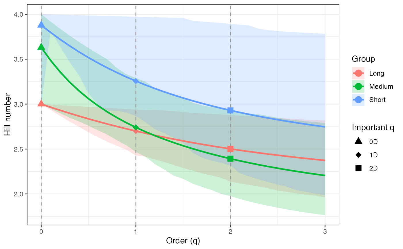
ggplot(hill_profile2_df, aes(x = q, y = mean,
color = group, fill = group)) +
geom_ribbon(aes(ymin = lower, ymax = upper), alpha = 0.2, color = NA) +
geom_line(linewidth = 1) +
geom_vline(xintercept = c(0, 1, 2), linetype = "dashed",
color = "grey60") +
geom_point(data = hill_points2_df, aes(shape = order_label),
size = 3, stroke = 1, inherit.aes = TRUE) +
scale_shape_manual(values = c(17, 18, 15), name = "Important q") +
labs(x = "Order (q)", y = "Hill number",
color = "Group", fill = "Group") +
theme_bw()
# Hill profile - BCa CIs ----
hill_profile2 <-
diversity.profile(pdata$CUAL, group = pdata$LNGS,
parameter = "hill", ci.type = "bca")
#> [1] "All values of t are equal to 3 \n Cannot calculate confidence intervals"
#> Warning: bca CI failed for component 1; using percentile CI.
hill_profile2
#> $Long
#> q observed mean lower upper
#> 1 0.0 3.000000 3.000000 3.000000 3.000000
#> 2 0.1 2.970041 2.963484 2.935089 2.996935
#> 3 0.2 2.940750 2.928275 2.872243 2.993713
#> 4 0.3 2.912153 2.894379 2.814506 2.990550
#> 5 0.4 2.884272 2.861794 2.758478 2.987375
#> 6 0.5 2.857124 2.830507 2.696544 2.982802
#> 7 0.6 2.830721 2.800498 2.650006 2.980991
#> 8 0.7 2.805073 2.771739 2.605210 2.977732
#> 9 0.8 2.780186 2.744201 2.556869 2.974310
#> 10 0.9 2.756060 2.717847 2.519271 2.970871
#> 11 1.0 2.732695 2.692639 2.462055 2.965921
#> 12 1.1 2.710085 2.668539 2.422841 2.962708
#> 13 1.2 2.688224 2.645505 2.410277 2.961612
#> 14 1.3 2.667101 2.623495 2.376388 2.958356
#> 15 1.4 2.646704 2.602466 2.344911 2.955094
#> 16 1.5 2.627019 2.582378 2.313303 2.951828
#> 17 1.6 2.608031 2.563189 2.265344 2.947898
#> 18 1.7 2.589722 2.544858 2.244240 2.944564
#> 19 1.8 2.572075 2.527345 2.221926 2.941449
#> 20 1.9 2.555070 2.510612 2.199733 2.938409
#> 21 2.0 2.538688 2.494621 2.147473 2.930663
#> 22 2.1 2.522908 2.479336 2.130369 2.926976
#> 23 2.2 2.507711 2.464723 2.127412 2.928886
#> 24 2.3 2.493075 2.450747 2.109897 2.925606
#> 25 2.4 2.478981 2.437377 2.096278 2.922327
#> 26 2.5 2.465409 2.424583 2.071867 2.915275
#> 27 2.6 2.452337 2.412335 2.063797 2.915778
#> 28 2.7 2.439748 2.400606 2.046616 2.906689
#> 29 2.8 2.427621 2.389369 2.032866 2.903510
#> 30 2.9 2.415938 2.378599 2.019115 2.903921
#> 31 3.0 2.404680 2.368272 2.005812 2.899450
#>
#> $Medium
#> q observed mean lower upper
#> 1 0.0 4.000000 3.619000 3.000000 4.000000
#> 2 0.1 3.775167 3.476264 2.950913 3.907938
#> 3 0.2 3.586424 3.350975 2.902339 3.822889
#> 4 0.3 3.427791 3.240771 2.856204 3.744454
#> 5 0.4 3.293906 3.143466 2.811608 3.672203
#> 6 0.5 3.180150 3.057121 2.765867 3.605693
#> 7 0.6 3.082659 2.980060 2.713960 3.544473
#> 8 0.7 2.998274 2.910866 2.658870 3.488104
#> 9 0.8 2.924454 2.848358 2.595904 3.430780
#> 10 0.9 2.859178 2.791559 2.526859 3.371489
#> 11 1.0 2.800853 2.739667 2.460082 3.271323
#> 12 1.1 2.748230 2.692024 2.405632 3.222461
#> 13 1.2 2.700330 2.648088 2.333804 3.176330
#> 14 1.3 2.656390 2.607414 2.271640 3.081676
#> 15 1.4 2.615811 2.569633 2.219938 3.047018
#> 16 1.5 2.578125 2.534436 2.174993 3.028985
#> 17 1.6 2.542961 2.501564 2.121365 2.989710
#> 18 1.7 2.510025 2.470797 2.081170 2.937736
#> 19 1.8 2.479080 2.441946 2.053267 2.918376
#> 20 1.9 2.449934 2.414849 2.000230 2.885359
#> 21 2.0 2.422430 2.389362 1.973701 2.877627
#> 22 2.1 2.396434 2.365360 1.942742 2.852153
#> 23 2.2 2.371835 2.342731 1.924305 2.840270
#> 24 2.3 2.348536 2.321375 1.903314 2.820106
#> 25 2.4 2.326451 2.301203 1.872879 2.810910
#> 26 2.5 2.305505 2.282131 1.840750 2.800566
#> 27 2.6 2.285629 2.264086 1.822221 2.792929
#> 28 2.7 2.266761 2.247000 1.805126 2.785276
#> 29 2.8 2.248843 2.230809 1.789084 2.776269
#> 30 2.9 2.231821 2.215457 1.774894 2.768542
#> 31 3.0 2.215647 2.200889 1.761344 2.759915
#>
#> $Short
#> q observed mean lower upper
#> 1 0.0 4.000000 3.869000 3.000000 4.000000
#> 2 0.1 3.933810 3.788600 3.830174 3.997186
#> 3 0.2 3.870196 3.712786 3.671165 3.994379
#> 4 0.3 3.809136 3.641430 3.522728 3.991579
#> 5 0.4 3.750595 3.574370 3.355476 3.988787
#> 6 0.5 3.694521 3.511417 3.227856 3.986001
#> 7 0.6 3.640856 3.452367 3.065308 3.983223
#> 8 0.7 3.589527 3.397005 2.989034 3.980453
#> 9 0.8 3.540459 3.345115 2.960386 3.977690
#> 10 0.9 3.493567 3.296479 2.943539 3.974936
#> 11 1.0 3.448767 3.250889 2.896553 3.972189
#> 12 1.1 3.405970 3.208141 2.853312 3.969451
#> 13 1.2 3.365087 3.168040 2.789734 3.966722
#> 14 1.3 3.326031 3.130403 2.730808 3.964001
#> 15 1.4 3.288713 3.095056 2.676150 3.961288
#> 16 1.5 3.253050 3.061838 2.625408 3.958585
#> 17 1.6 3.218958 3.030597 2.534687 3.955890
#> 18 1.7 3.186359 3.001191 2.501868 3.953205
#> 19 1.8 3.155176 2.973490 2.472077 3.950529
#> 20 1.9 3.125338 2.947372 2.428298 3.947863
#> 21 2.0 3.096774 2.922726 2.380165 3.945205
#> 22 2.1 3.069420 2.899446 2.277887 3.906120
#> 23 2.2 3.043214 2.877438 2.253808 3.897045
#> 24 2.3 3.018098 2.856612 2.231544 3.876801
#> 25 2.4 2.994016 2.836888 2.210903 3.871853
#> 26 2.5 2.970917 2.818189 2.191717 3.866947
#> 27 2.6 2.948751 2.800447 2.086670 3.862084
#> 28 2.7 2.927474 2.783597 2.041816 3.798686
#> 29 2.8 2.907041 2.767580 2.021941 3.793312
#> 30 2.9 2.887412 2.752342 2.003460 3.788060
#> 31 3.0 2.868549 2.737833 1.986254 3.782930
#>
#> attr(,"R")
#> [1] 1000
#> attr(,"conf")
#> [1] 0.95
#> attr(,"parameter")
#> [1] "hill"
#> attr(,"ci.type")
#> [1] "bca"
hill_profile2_df <- dplyr::bind_rows(hill_profile2, .id = "group")
hill_points2_df <- hill_profile2_df %>%
filter(q %in% important_q) %>%
mutate(order_label = factor(q, levels = important_q,
labels = important_labels))
ggplot(hill_profile2_df, aes(x = q, y = mean,
color = group, fill = group)) +
geom_ribbon(aes(ymin = lower, ymax = upper), alpha = 0.2, color = NA) +
geom_line(linewidth = 1) +
geom_vline(xintercept = c(0, 1, 2), linetype = "dashed",
color = "grey60") +
geom_point(data = hill_points2_df, aes(shape = order_label),
size = 3, stroke = 1, inherit.aes = TRUE) +
scale_shape_manual(values = c(17, 18, 15), name = "Important q") +
labs(x = "Order (q)", y = "Hill number",
color = "Group", fill = "Group") +
theme_bw()
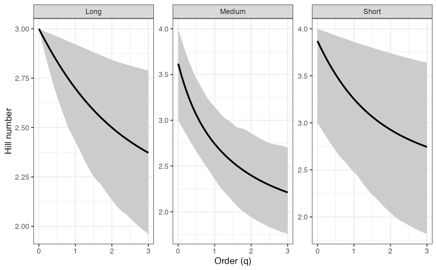
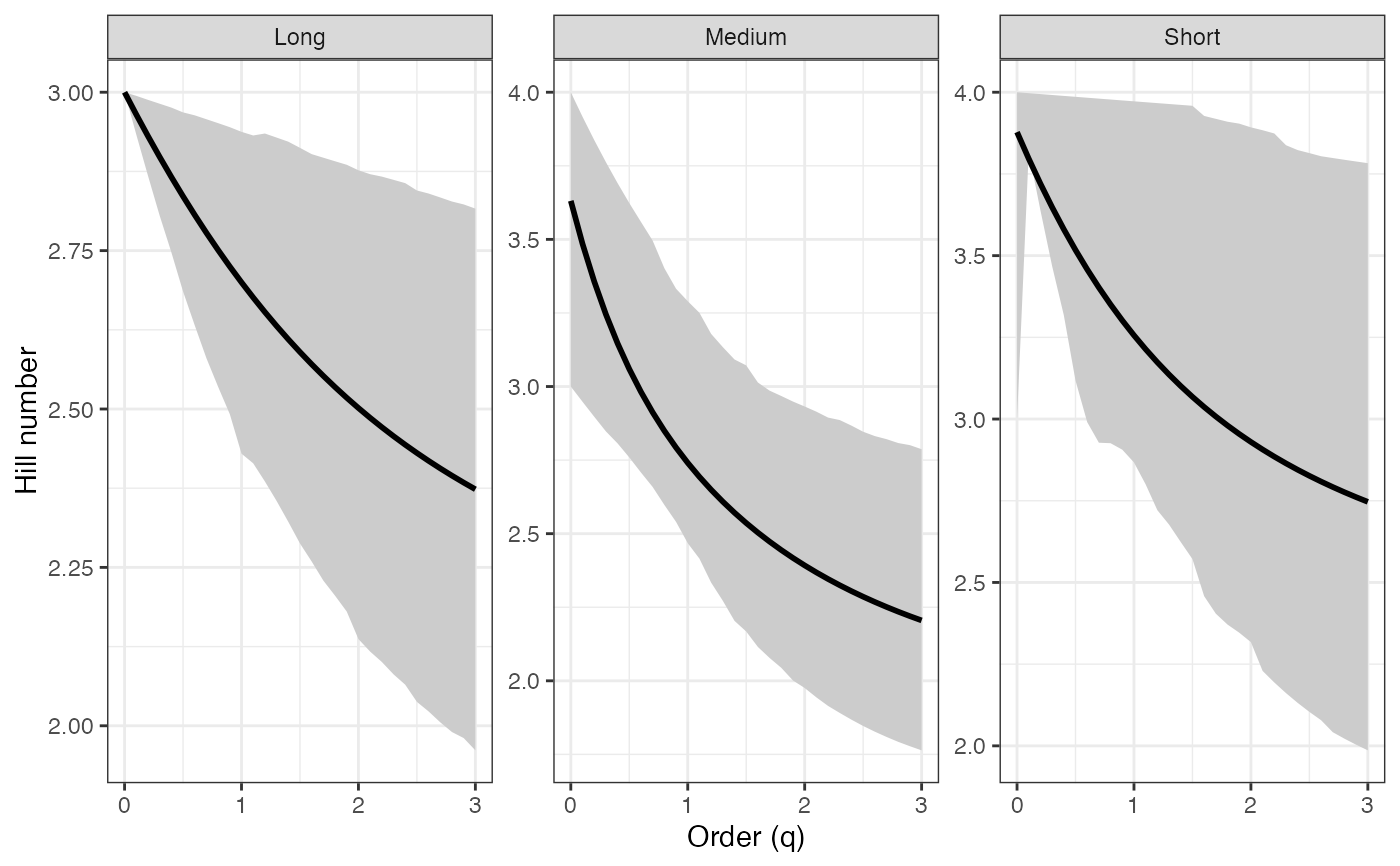
 ggplot(hill_profile2_df, aes(x = q, y = mean)) +
geom_ribbon(aes(ymin = lower, ymax = upper), fill = "grey80") +
geom_line(color = "black", linewidth = 1) +
facet_wrap(~ group, scales = "free_y") +
labs(x = "Order (q)", y = "Hill number") +
theme_bw()
ggplot(hill_profile2_df, aes(x = q, y = mean)) +
geom_ribbon(aes(ymin = lower, ymax = upper), fill = "grey80") +
geom_line(color = "black", linewidth = 1) +
facet_wrap(~ group, scales = "free_y") +
labs(x = "Order (q)", y = "Hill number") +
theme_bw()
 # Rényi profile - BCa CIs ----
renyi_profile2 <-
diversity.profile(pdata$CUAL, group = pdata$LNGS,
parameter = "renyi", ci.type = "bca")
#> [1] "All values of t are equal to 1.09861228866811 \n Cannot calculate confidence intervals"
#> Warning: bca CI failed for component 1; using percentile CI.
renyi_profile2
#> $Long
#> q observed mean lower upper
#> 1 0.0 1.0986123 1.0986123 1.0986123 1.098612
#> 2 0.1 1.0885756 1.0866342 1.0741825 1.096309
#> 3 0.2 1.0786646 1.0748681 1.0493698 1.093813
#> 4 0.3 1.0688928 1.0633362 1.0262299 1.091460
#> 5 0.4 1.0592726 1.0520574 1.0031925 1.089139
#> 6 0.5 1.0498155 1.0410473 0.9803805 1.086567
#> 7 0.6 1.0405315 1.0303187 0.9603003 1.084595
#> 8 0.7 1.0314297 1.0198811 0.9396717 1.082374
#> 9 0.8 1.0225177 1.0097416 0.9207653 1.080113
#> 10 0.9 1.0138021 0.9999048 0.9032084 1.077833
#> 11 1.0 1.0052882 0.9903729 0.8823320 1.073935
#> 12 1.1 0.9969801 0.9811463 0.8707489 1.072457
#> 13 1.2 0.9888807 0.9722238 0.8571959 1.071787
#> 14 1.3 0.9809920 0.9636025 0.8410913 1.069775
#> 15 1.4 0.9733151 0.9552783 0.8272766 1.067787
#> 16 1.5 0.9658499 0.9472461 0.8144799 1.065631
#> 17 1.6 0.9585956 0.9394999 0.8010208 1.063164
#> 18 1.7 0.9515507 0.9320328 0.7846121 1.060285
#> 19 1.8 0.9447130 0.9248377 0.7721263 1.058135
#> 20 1.9 0.9380796 0.9179067 0.7605096 1.055828
#> 21 2.0 0.9316472 0.9112317 0.7470429 1.044545
#> 22 2.1 0.9254122 0.9048045 0.7384205 1.042274
#> 23 2.2 0.9193702 0.8986166 0.7302797 1.045710
#> 24 2.3 0.9135169 0.8926595 0.7225839 1.043535
#> 25 2.4 0.9078477 0.8869248 0.7152995 1.041354
#> 26 2.5 0.9023576 0.8814041 0.7023542 1.036813
#> 27 2.6 0.8970416 0.8760890 0.6999051 1.037546
#> 28 2.7 0.8918947 0.8709715 0.6900979 1.034211
#> 29 2.8 0.8869118 0.8660436 0.6829793 1.032025
#> 30 2.9 0.8820876 0.8612976 0.6778175 1.032759
#> 31 3.0 0.8774170 0.8567259 0.6702424 1.027713
#>
#> $Medium
#> q observed mean lower upper
#> 1 0.0 1.3862944 1.2792766 1.0986123 1.386294
#> 2 0.1 1.3284446 1.2408711 1.0806903 1.369794
#> 3 0.2 1.2771555 1.2054497 1.0625981 1.353677
#> 4 0.3 1.2319160 1.1728761 1.0453591 1.337960
#> 5 0.4 1.1920742 1.1429453 1.0275574 1.322654
#> 6 0.5 1.1569284 1.1154174 1.0086792 1.307768
#> 7 0.6 1.1257925 1.0900448 0.9897522 1.293307
#> 8 0.7 1.0980367 1.0665897 0.9717405 1.269920
#> 9 0.8 1.0731077 1.0448338 0.9500916 1.240227
#> 10 0.9 1.0505342 1.0245838 0.9262639 1.215429
#> 11 1.0 1.0299241 1.0056716 0.9007170 1.193408
#> 12 1.1 1.0109570 0.9879533 0.8791745 1.171583
#> 13 1.2 0.9933740 0.9713067 0.8488514 1.152860
#> 14 1.3 0.9769680 0.9556282 0.8160699 1.132041
#> 15 1.4 0.9615743 0.9408302 0.7899261 1.116816
#> 16 1.5 0.9470625 0.9268380 0.7735497 1.112612
#> 17 1.6 0.9333293 0.9135880 0.7527004 1.098676
#> 18 1.7 0.9202928 0.9010251 0.7334819 1.091484
#> 19 1.8 0.9078876 0.8891013 0.7179903 1.084420
#> 20 1.9 0.8960613 0.8777744 0.7018772 1.076342
#> 21 2.0 0.8847711 0.8670068 0.6892831 1.070088
#> 22 2.1 0.8739819 0.8567647 0.6737503 1.064010
#> 23 2.2 0.8636641 0.8470174 0.6620047 1.058148
#> 24 2.3 0.8537922 0.8377366 0.6509533 1.052882
#> 25 2.4 0.8443440 0.8288966 0.6405591 1.048054
#> 26 2.5 0.8352998 0.8204730 0.6307849 1.043387
#> 27 2.6 0.8266413 0.8124435 0.6215944 1.038783
#> 28 2.7 0.8183519 0.8047868 0.6129520 1.034196
#> 29 2.8 0.8104158 0.7974832 0.6032391 1.027949
#> 30 2.9 0.8028180 0.7905140 0.5956450 1.024301
#> 31 3.0 0.7955444 0.7838615 0.5885164 1.020962
#>
#> $Short
#> q observed mean lower upper
#> 1 0.0 1.386294 1.3490656 0.6931472 1.386294
#> 2 0.1 1.369609 1.3284579 1.3374228 1.385591
#> 3 0.2 1.353305 1.3084604 1.2897519 1.384888
#> 4 0.3 1.337402 1.2891189 1.2330363 1.384187
#> 5 0.4 1.321914 1.2704669 1.1840225 1.383487
#> 6 0.5 1.306851 1.2525262 1.1308601 1.382788
#> 7 0.6 1.292219 1.2353083 1.0923031 1.382091
#> 8 0.7 1.278021 1.2188153 1.0741728 1.381396
#> 9 0.8 1.264256 1.2030418 1.0706283 1.380701
#> 10 0.9 1.250923 1.1879759 1.0629474 1.380009
#> 11 1.0 1.238017 1.1736008 1.0533373 1.379317
#> 12 1.1 1.225530 1.1598958 1.0290125 1.378628
#> 13 1.2 1.213454 1.1468375 1.0058584 1.377940
#> 14 1.3 1.201780 1.1344007 0.9779543 1.377254
#> 15 1.4 1.190496 1.1225588 0.9612580 1.376569
#> 16 1.5 1.179593 1.1112848 0.9431998 1.375887
#> 17 1.6 1.169058 1.1005515 0.8993946 1.375206
#> 18 1.7 1.158879 1.0903321 0.8829979 1.374527
#> 19 1.8 1.149044 1.0806002 0.8719362 1.373850
#> 20 1.9 1.139542 1.0713303 0.8611926 1.373174
#> 21 2.0 1.130361 1.0624977 0.8507761 1.372501
#> 22 2.1 1.121489 1.0540787 0.8328713 1.371830
#> 23 2.2 1.112914 1.0460507 0.8234196 1.371161
#> 24 2.3 1.104627 1.0383921 0.8070595 1.370493
#> 25 2.4 1.096616 1.0310826 0.7950799 1.367769
#> 26 2.5 1.088871 1.0241027 0.7846855 1.366104
#> 27 2.6 1.081382 1.0174341 0.7764957 1.358751
#> 28 2.7 1.074140 1.0110596 0.7237967 1.349958
#> 29 2.8 1.067136 1.0049630 0.7097815 1.348720
#> 30 2.9 1.060361 0.9991289 0.6998077 1.347491
#> 31 3.0 1.053806 0.9935429 0.6905498 1.346273
#>
#> attr(,"R")
#> [1] 1000
#> attr(,"conf")
#> [1] 0.95
#> attr(,"parameter")
#> [1] "renyi"
#> attr(,"ci.type")
#> [1] "bca"
renyi_profile2_df <- dplyr::bind_rows(renyi_profile2, .id = "group")
renyi_points2_df <- renyi_profile2_df %>%
filter(q %in% important_q) %>%
mutate(order_label = factor(q, levels = important_q,
labels = important_labels))
ggplot(renyi_profile2_df, aes(x = q, y = mean,
color = group, fill = group)) +
geom_ribbon(aes(ymin = lower, ymax = upper), alpha = 0.2, color = NA) +
geom_line(linewidth = 1) +
geom_vline(xintercept = c(0, 1, 2), linetype = "dashed",
color = "grey60") +
geom_point(data = renyi_points2_df, aes(shape = order_label),
size = 3, stroke = 1, inherit.aes = TRUE) +
scale_shape_manual(values = c(17, 18, 15), name = "Important q") +
labs(x = "Order (q)", y = "Hill number",
color = "Group", fill = "Group") +
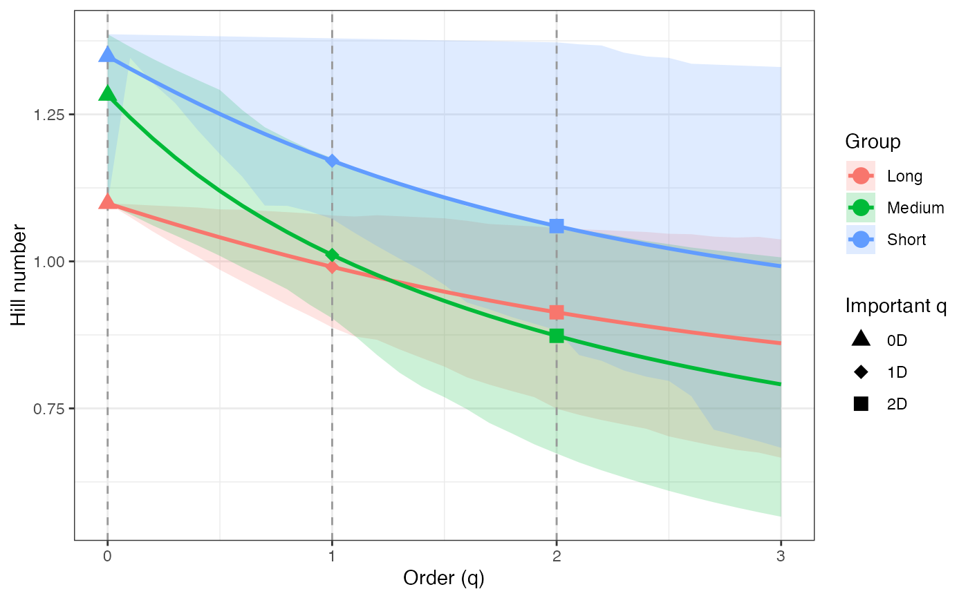
theme_bw()
# Rényi profile - BCa CIs ----
renyi_profile2 <-
diversity.profile(pdata$CUAL, group = pdata$LNGS,
parameter = "renyi", ci.type = "bca")
#> [1] "All values of t are equal to 1.09861228866811 \n Cannot calculate confidence intervals"
#> Warning: bca CI failed for component 1; using percentile CI.
renyi_profile2
#> $Long
#> q observed mean lower upper
#> 1 0.0 1.0986123 1.0986123 1.0986123 1.098612
#> 2 0.1 1.0885756 1.0866342 1.0741825 1.096309
#> 3 0.2 1.0786646 1.0748681 1.0493698 1.093813
#> 4 0.3 1.0688928 1.0633362 1.0262299 1.091460
#> 5 0.4 1.0592726 1.0520574 1.0031925 1.089139
#> 6 0.5 1.0498155 1.0410473 0.9803805 1.086567
#> 7 0.6 1.0405315 1.0303187 0.9603003 1.084595
#> 8 0.7 1.0314297 1.0198811 0.9396717 1.082374
#> 9 0.8 1.0225177 1.0097416 0.9207653 1.080113
#> 10 0.9 1.0138021 0.9999048 0.9032084 1.077833
#> 11 1.0 1.0052882 0.9903729 0.8823320 1.073935
#> 12 1.1 0.9969801 0.9811463 0.8707489 1.072457
#> 13 1.2 0.9888807 0.9722238 0.8571959 1.071787
#> 14 1.3 0.9809920 0.9636025 0.8410913 1.069775
#> 15 1.4 0.9733151 0.9552783 0.8272766 1.067787
#> 16 1.5 0.9658499 0.9472461 0.8144799 1.065631
#> 17 1.6 0.9585956 0.9394999 0.8010208 1.063164
#> 18 1.7 0.9515507 0.9320328 0.7846121 1.060285
#> 19 1.8 0.9447130 0.9248377 0.7721263 1.058135
#> 20 1.9 0.9380796 0.9179067 0.7605096 1.055828
#> 21 2.0 0.9316472 0.9112317 0.7470429 1.044545
#> 22 2.1 0.9254122 0.9048045 0.7384205 1.042274
#> 23 2.2 0.9193702 0.8986166 0.7302797 1.045710
#> 24 2.3 0.9135169 0.8926595 0.7225839 1.043535
#> 25 2.4 0.9078477 0.8869248 0.7152995 1.041354
#> 26 2.5 0.9023576 0.8814041 0.7023542 1.036813
#> 27 2.6 0.8970416 0.8760890 0.6999051 1.037546
#> 28 2.7 0.8918947 0.8709715 0.6900979 1.034211
#> 29 2.8 0.8869118 0.8660436 0.6829793 1.032025
#> 30 2.9 0.8820876 0.8612976 0.6778175 1.032759
#> 31 3.0 0.8774170 0.8567259 0.6702424 1.027713
#>
#> $Medium
#> q observed mean lower upper
#> 1 0.0 1.3862944 1.2792766 1.0986123 1.386294
#> 2 0.1 1.3284446 1.2408711 1.0806903 1.369794
#> 3 0.2 1.2771555 1.2054497 1.0625981 1.353677
#> 4 0.3 1.2319160 1.1728761 1.0453591 1.337960
#> 5 0.4 1.1920742 1.1429453 1.0275574 1.322654
#> 6 0.5 1.1569284 1.1154174 1.0086792 1.307768
#> 7 0.6 1.1257925 1.0900448 0.9897522 1.293307
#> 8 0.7 1.0980367 1.0665897 0.9717405 1.269920
#> 9 0.8 1.0731077 1.0448338 0.9500916 1.240227
#> 10 0.9 1.0505342 1.0245838 0.9262639 1.215429
#> 11 1.0 1.0299241 1.0056716 0.9007170 1.193408
#> 12 1.1 1.0109570 0.9879533 0.8791745 1.171583
#> 13 1.2 0.9933740 0.9713067 0.8488514 1.152860
#> 14 1.3 0.9769680 0.9556282 0.8160699 1.132041
#> 15 1.4 0.9615743 0.9408302 0.7899261 1.116816
#> 16 1.5 0.9470625 0.9268380 0.7735497 1.112612
#> 17 1.6 0.9333293 0.9135880 0.7527004 1.098676
#> 18 1.7 0.9202928 0.9010251 0.7334819 1.091484
#> 19 1.8 0.9078876 0.8891013 0.7179903 1.084420
#> 20 1.9 0.8960613 0.8777744 0.7018772 1.076342
#> 21 2.0 0.8847711 0.8670068 0.6892831 1.070088
#> 22 2.1 0.8739819 0.8567647 0.6737503 1.064010
#> 23 2.2 0.8636641 0.8470174 0.6620047 1.058148
#> 24 2.3 0.8537922 0.8377366 0.6509533 1.052882
#> 25 2.4 0.8443440 0.8288966 0.6405591 1.048054
#> 26 2.5 0.8352998 0.8204730 0.6307849 1.043387
#> 27 2.6 0.8266413 0.8124435 0.6215944 1.038783
#> 28 2.7 0.8183519 0.8047868 0.6129520 1.034196
#> 29 2.8 0.8104158 0.7974832 0.6032391 1.027949
#> 30 2.9 0.8028180 0.7905140 0.5956450 1.024301
#> 31 3.0 0.7955444 0.7838615 0.5885164 1.020962
#>
#> $Short
#> q observed mean lower upper
#> 1 0.0 1.386294 1.3490656 0.6931472 1.386294
#> 2 0.1 1.369609 1.3284579 1.3374228 1.385591
#> 3 0.2 1.353305 1.3084604 1.2897519 1.384888
#> 4 0.3 1.337402 1.2891189 1.2330363 1.384187
#> 5 0.4 1.321914 1.2704669 1.1840225 1.383487
#> 6 0.5 1.306851 1.2525262 1.1308601 1.382788
#> 7 0.6 1.292219 1.2353083 1.0923031 1.382091
#> 8 0.7 1.278021 1.2188153 1.0741728 1.381396
#> 9 0.8 1.264256 1.2030418 1.0706283 1.380701
#> 10 0.9 1.250923 1.1879759 1.0629474 1.380009
#> 11 1.0 1.238017 1.1736008 1.0533373 1.379317
#> 12 1.1 1.225530 1.1598958 1.0290125 1.378628
#> 13 1.2 1.213454 1.1468375 1.0058584 1.377940
#> 14 1.3 1.201780 1.1344007 0.9779543 1.377254
#> 15 1.4 1.190496 1.1225588 0.9612580 1.376569
#> 16 1.5 1.179593 1.1112848 0.9431998 1.375887
#> 17 1.6 1.169058 1.1005515 0.8993946 1.375206
#> 18 1.7 1.158879 1.0903321 0.8829979 1.374527
#> 19 1.8 1.149044 1.0806002 0.8719362 1.373850
#> 20 1.9 1.139542 1.0713303 0.8611926 1.373174
#> 21 2.0 1.130361 1.0624977 0.8507761 1.372501
#> 22 2.1 1.121489 1.0540787 0.8328713 1.371830
#> 23 2.2 1.112914 1.0460507 0.8234196 1.371161
#> 24 2.3 1.104627 1.0383921 0.8070595 1.370493
#> 25 2.4 1.096616 1.0310826 0.7950799 1.367769
#> 26 2.5 1.088871 1.0241027 0.7846855 1.366104
#> 27 2.6 1.081382 1.0174341 0.7764957 1.358751
#> 28 2.7 1.074140 1.0110596 0.7237967 1.349958
#> 29 2.8 1.067136 1.0049630 0.7097815 1.348720
#> 30 2.9 1.060361 0.9991289 0.6998077 1.347491
#> 31 3.0 1.053806 0.9935429 0.6905498 1.346273
#>
#> attr(,"R")
#> [1] 1000
#> attr(,"conf")
#> [1] 0.95
#> attr(,"parameter")
#> [1] "renyi"
#> attr(,"ci.type")
#> [1] "bca"
renyi_profile2_df <- dplyr::bind_rows(renyi_profile2, .id = "group")
renyi_points2_df <- renyi_profile2_df %>%
filter(q %in% important_q) %>%
mutate(order_label = factor(q, levels = important_q,
labels = important_labels))
ggplot(renyi_profile2_df, aes(x = q, y = mean,
color = group, fill = group)) +
geom_ribbon(aes(ymin = lower, ymax = upper), alpha = 0.2, color = NA) +
geom_line(linewidth = 1) +
geom_vline(xintercept = c(0, 1, 2), linetype = "dashed",
color = "grey60") +
geom_point(data = renyi_points2_df, aes(shape = order_label),
size = 3, stroke = 1, inherit.aes = TRUE) +
scale_shape_manual(values = c(17, 18, 15), name = "Important q") +
labs(x = "Order (q)", y = "Hill number",
color = "Group", fill = "Group") +
theme_bw()
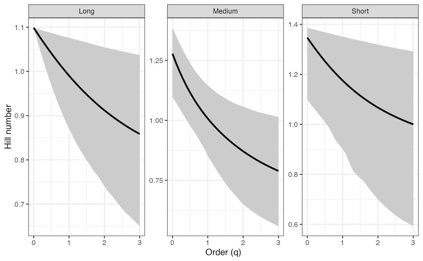
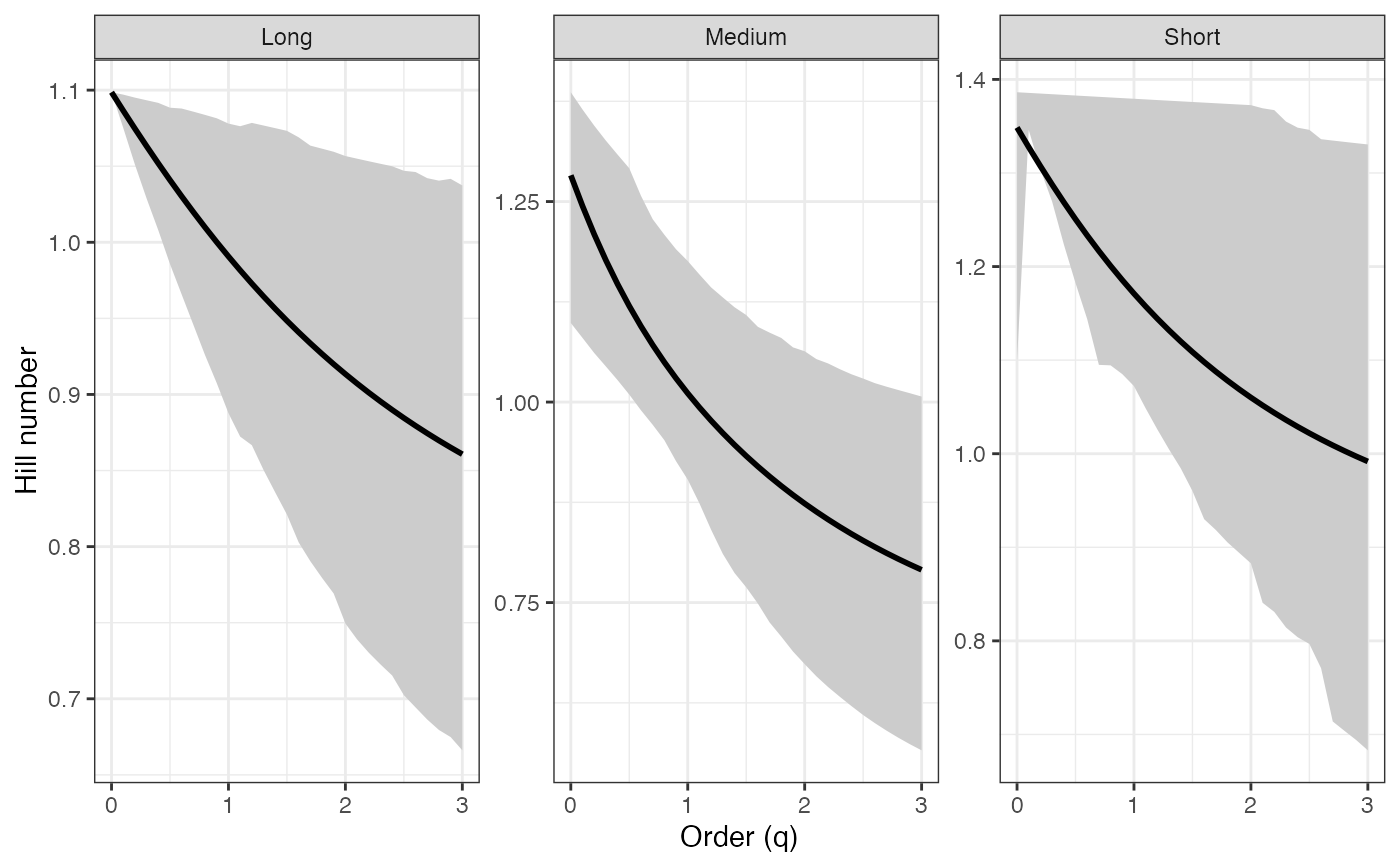
 ggplot(renyi_profile2_df, aes(x = q, y = mean)) +
geom_ribbon(aes(ymin = lower, ymax = upper), fill = "grey80") +
geom_line(color = "black", linewidth = 1) +
facet_wrap(~ group, scales = "free_y") +
labs(x = "Order (q)", y = "Hill number") +
theme_bw()
ggplot(renyi_profile2_df, aes(x = q, y = mean)) +
geom_ribbon(aes(ymin = lower, ymax = upper), fill = "grey80") +
geom_line(color = "black", linewidth = 1) +
facet_wrap(~ group, scales = "free_y") +
labs(x = "Order (q)", y = "Hill number") +
theme_bw()
 # Tsallis profile - BCa CIs ----
tsallis_profile2 <-
diversity.profile(pdata$CUAL, group = pdata$LNGS,
parameter = "tsallis", ci.type = "bca")
#> [1] "All values of t are equal to 2 \n Cannot calculate confidence intervals"
#> Warning: bca CI failed for component 1; using percentile CI.
tsallis_profile2
#> $Long
#> q observed mean lower upper
#> 1 0.0 2.0000000 2.0000000 2.0000000 2.0000000
#> 2 0.1 1.8485612 1.8420577 1.8155862 1.8722238
#> 3 0.2 1.7126236 1.7014029 1.6509674 1.7544649
#> 4 0.3 1.5903508 1.5757981 1.5093622 1.6459554
#> 5 0.4 1.4801432 1.4633278 1.3875941 1.5458713
#> 6 0.5 1.3806058 1.3623482 1.2769199 1.4532412
#> 7 0.6 1.2905205 1.2714459 1.1872889 1.3681665
#> 8 0.7 1.2088223 1.1894028 1.1019222 1.2892947
#> 9 0.8 1.1345790 1.1151671 1.0264221 1.2163347
#> 10 0.9 1.0669734 1.0478283 0.9586620 1.1487914
#> 11 1.0 1.0052882 0.9865965 0.8967229 1.0861389
#> 12 1.1 0.9488928 0.9307854 0.8440571 1.0281575
#> 13 1.2 0.8972324 0.8797969 0.8036290 0.9749215
#> 14 1.3 0.8498176 0.8331088 0.7621337 0.9248429
#> 15 1.4 0.8062167 0.7902644 0.7209079 0.8782757
#> 16 1.5 0.7660477 0.7508630 0.6832590 0.8348762
#> 17 1.6 0.7289728 0.7145528 0.6482739 0.7944513
#> 18 1.7 0.6946920 0.6810239 0.6163014 0.7568373
#> 19 1.8 0.6629392 0.6500027 0.5877176 0.7218190
#> 20 1.9 0.6334774 0.6212475 0.5616582 0.6891216
#> 21 2.0 0.6060957 0.5945440 0.5320216 0.6565106
#> 22 2.1 0.5806057 0.5697020 0.5107226 0.6280166
#> 23 2.2 0.5568392 0.5465523 0.4928750 0.6021501
#> 24 2.3 0.5346455 0.5249439 0.4733925 0.5770620
#> 25 2.4 0.5138895 0.5047421 0.4557913 0.5535482
#> 26 2.5 0.4944499 0.4858262 0.4392279 0.5311821
#> 27 2.6 0.4762176 0.4680882 0.4244539 0.5106728
#> 28 2.7 0.4590941 0.4514308 0.4090547 0.4910568
#> 29 2.8 0.4429909 0.4357666 0.3954328 0.4728135
#> 30 2.9 0.4278278 0.4210167 0.3829694 0.4557151
#> 31 3.0 0.4135320 0.4071098 0.3709220 0.4394392
#>
#> $Medium
#> q observed mean lower upper
#> 1 0.0 3.0000000 2.6330000 2.0000000 3.0000000
#> 2 0.1 2.5617123 2.3091337 1.8258798 2.6774933
#> 3 0.2 2.2224763 2.0471558 1.6720411 2.4035272
#> 4 0.3 1.9552854 1.8322403 1.5364321 2.1698269
#> 5 0.4 1.7411443 1.6535741 1.4159320 1.9690901
#> 6 0.5 1.5665950 1.5031963 1.3088279 1.7943247
#> 7 0.6 1.4220235 1.3751853 1.2134000 1.6400907
#> 8 0.7 1.3004971 1.2650891 1.1253855 1.5041263
#> 9 0.8 1.1969637 1.1695220 1.0406892 1.3780581
#> 10 0.9 1.1076994 1.0858793 0.9669214 1.2718320
#> 11 1.0 1.0299241 1.0121331 0.9002561 1.1812705
#> 12 1.1 0.9615347 0.9466857 0.8355431 1.0968625
#> 13 1.2 0.9009177 0.8882634 0.7789062 1.0208339
#> 14 1.3 0.8468176 0.8358396 0.7248090 0.9549525
#> 15 1.4 0.7982434 0.7885775 0.6827669 0.8982371
#> 16 1.5 0.7544018 0.7457883 0.6422783 0.8476669
#> 17 1.6 0.7146493 0.7068994 0.6039248 0.7979375
#> 18 1.7 0.6784574 0.6714309 0.5687863 0.7560305
#> 19 1.8 0.6453869 0.6389771 0.5399460 0.7185627
#> 20 1.9 0.6150691 0.6091927 0.5129420 0.6832663
#> 21 2.0 0.5871914 0.5817816 0.4903549 0.6515292
#> 22 2.1 0.5614865 0.5564889 0.4683169 0.6213434
#> 23 2.2 0.5377246 0.5330933 0.4488865 0.5938201
#> 24 2.3 0.5157061 0.5114024 0.4310735 0.5686240
#> 25 2.4 0.4952573 0.4912477 0.4146904 0.5448343
#> 26 2.5 0.4762260 0.4724813 0.3995760 0.5227557
#> 27 2.6 0.4584783 0.4549728 0.3855906 0.5020808
#> 28 2.7 0.4418959 0.4386070 0.3726134 0.4827549
#> 29 2.8 0.4263738 0.4232815 0.3604535 0.4646499
#> 30 2.9 0.4118190 0.4089054 0.3490276 0.4476658
#> 31 3.0 0.3981481 0.3953974 0.3385268 0.4319513
#>
#> $Short
#> q observed mean lower upper
#> 1 0.0 3.0000000 2.8700000 2.0000000 3.0000000
#> 2 0.1 2.7003331 2.5718026 2.6200828 2.7555529
#> 3 0.2 2.4405950 2.3164713 2.3062899 2.5350311
#> 4 0.3 2.2146076 2.0966623 2.0453715 2.3358938
#> 5 0.4 2.0172417 1.9064405 1.8269534 2.1558838
#> 6 0.5 1.8442276 1.7409876 1.6315503 1.9929944
#> 7 0.6 1.6920012 1.5963736 1.4767373 1.8454410
#> 8 0.7 1.5575795 1.4693789 1.3274550 1.7116355
#> 9 0.8 1.4384586 1.3573531 1.2387314 1.5901636
#> 10 0.9 1.3325309 1.2581046 1.1518215 1.4797653
#> 11 1.0 1.2380168 1.1698130 1.0722551 1.3793174
#> 12 1.1 1.1534096 1.0909590 1.0020689 1.2878177
#> 13 1.2 1.0774297 1.0202692 0.9275343 1.2043718
#> 14 1.3 1.0089869 0.9566715 0.8671548 1.1281808
#> 15 1.4 0.9471496 0.8992596 0.8130914 1.0585306
#> 16 1.5 0.8911198 0.8472636 0.7625994 0.9947826
#> 17 1.6 0.8402110 0.8000273 0.7148572 0.9347007
#> 18 1.7 0.7938317 0.7569890 0.6778582 0.8807360
#> 19 1.8 0.7514702 0.7176659 0.6447868 0.8312592
#> 20 1.9 0.7126828 0.6816416 0.6141589 0.7858330
#> 21 2.0 0.6770833 0.6485556 0.5868056 0.7440659
#> 22 2.1 0.6443352 0.6180947 0.5538302 0.7019577
#> 23 2.2 0.6141439 0.5899859 0.5299181 0.6668697
#> 24 2.3 0.5862509 0.5639906 0.5023573 0.6345963
#> 25 2.4 0.5604291 0.5398991 0.4830384 0.6047168
#> 26 2.5 0.5364780 0.5175273 0.4650122 0.5770162
#> 27 2.6 0.5142206 0.4967123 0.4479557 0.5513011
#> 28 2.7 0.4934997 0.4773104 0.4277144 0.5273974
#> 29 2.8 0.4741760 0.4591935 0.4134473 0.5051482
#> 30 2.9 0.4561251 0.4422482 0.4000222 0.4844119
#> 31 3.0 0.4392361 0.4263730 0.3873698 0.4650608
#>
#> attr(,"R")
#> [1] 1000
#> attr(,"conf")
#> [1] 0.95
#> attr(,"parameter")
#> [1] "tsallis"
#> attr(,"ci.type")
#> [1] "bca"
tsallis_profile2_df <- dplyr::bind_rows(tsallis_profile2, .id = "group")
tsallis_points2_df <- tsallis_profile2_df %>%
filter(q %in% important_q) %>%
mutate(order_label = factor(q, levels = important_q,
labels = important_labels))
ggplot(tsallis_profile2_df, aes(x = q, y = mean,
color = group, fill = group)) +
geom_ribbon(aes(ymin = lower, ymax = upper), alpha = 0.2, color = NA) +
geom_line(linewidth = 1) +
geom_vline(xintercept = c(0, 1, 2), linetype = "dashed",
color = "grey60") +
geom_point(data = tsallis_points2_df, aes(shape = order_label),
size = 3, stroke = 1, inherit.aes = TRUE) +
scale_shape_manual(values = c(17, 18, 15), name = "Important q") +
labs(x = "Order (q)", y = "Hill number",
color = "Group", fill = "Group") +
theme_bw()
# Tsallis profile - BCa CIs ----
tsallis_profile2 <-
diversity.profile(pdata$CUAL, group = pdata$LNGS,
parameter = "tsallis", ci.type = "bca")
#> [1] "All values of t are equal to 2 \n Cannot calculate confidence intervals"
#> Warning: bca CI failed for component 1; using percentile CI.
tsallis_profile2
#> $Long
#> q observed mean lower upper
#> 1 0.0 2.0000000 2.0000000 2.0000000 2.0000000
#> 2 0.1 1.8485612 1.8420577 1.8155862 1.8722238
#> 3 0.2 1.7126236 1.7014029 1.6509674 1.7544649
#> 4 0.3 1.5903508 1.5757981 1.5093622 1.6459554
#> 5 0.4 1.4801432 1.4633278 1.3875941 1.5458713
#> 6 0.5 1.3806058 1.3623482 1.2769199 1.4532412
#> 7 0.6 1.2905205 1.2714459 1.1872889 1.3681665
#> 8 0.7 1.2088223 1.1894028 1.1019222 1.2892947
#> 9 0.8 1.1345790 1.1151671 1.0264221 1.2163347
#> 10 0.9 1.0669734 1.0478283 0.9586620 1.1487914
#> 11 1.0 1.0052882 0.9865965 0.8967229 1.0861389
#> 12 1.1 0.9488928 0.9307854 0.8440571 1.0281575
#> 13 1.2 0.8972324 0.8797969 0.8036290 0.9749215
#> 14 1.3 0.8498176 0.8331088 0.7621337 0.9248429
#> 15 1.4 0.8062167 0.7902644 0.7209079 0.8782757
#> 16 1.5 0.7660477 0.7508630 0.6832590 0.8348762
#> 17 1.6 0.7289728 0.7145528 0.6482739 0.7944513
#> 18 1.7 0.6946920 0.6810239 0.6163014 0.7568373
#> 19 1.8 0.6629392 0.6500027 0.5877176 0.7218190
#> 20 1.9 0.6334774 0.6212475 0.5616582 0.6891216
#> 21 2.0 0.6060957 0.5945440 0.5320216 0.6565106
#> 22 2.1 0.5806057 0.5697020 0.5107226 0.6280166
#> 23 2.2 0.5568392 0.5465523 0.4928750 0.6021501
#> 24 2.3 0.5346455 0.5249439 0.4733925 0.5770620
#> 25 2.4 0.5138895 0.5047421 0.4557913 0.5535482
#> 26 2.5 0.4944499 0.4858262 0.4392279 0.5311821
#> 27 2.6 0.4762176 0.4680882 0.4244539 0.5106728
#> 28 2.7 0.4590941 0.4514308 0.4090547 0.4910568
#> 29 2.8 0.4429909 0.4357666 0.3954328 0.4728135
#> 30 2.9 0.4278278 0.4210167 0.3829694 0.4557151
#> 31 3.0 0.4135320 0.4071098 0.3709220 0.4394392
#>
#> $Medium
#> q observed mean lower upper
#> 1 0.0 3.0000000 2.6330000 2.0000000 3.0000000
#> 2 0.1 2.5617123 2.3091337 1.8258798 2.6774933
#> 3 0.2 2.2224763 2.0471558 1.6720411 2.4035272
#> 4 0.3 1.9552854 1.8322403 1.5364321 2.1698269
#> 5 0.4 1.7411443 1.6535741 1.4159320 1.9690901
#> 6 0.5 1.5665950 1.5031963 1.3088279 1.7943247
#> 7 0.6 1.4220235 1.3751853 1.2134000 1.6400907
#> 8 0.7 1.3004971 1.2650891 1.1253855 1.5041263
#> 9 0.8 1.1969637 1.1695220 1.0406892 1.3780581
#> 10 0.9 1.1076994 1.0858793 0.9669214 1.2718320
#> 11 1.0 1.0299241 1.0121331 0.9002561 1.1812705
#> 12 1.1 0.9615347 0.9466857 0.8355431 1.0968625
#> 13 1.2 0.9009177 0.8882634 0.7789062 1.0208339
#> 14 1.3 0.8468176 0.8358396 0.7248090 0.9549525
#> 15 1.4 0.7982434 0.7885775 0.6827669 0.8982371
#> 16 1.5 0.7544018 0.7457883 0.6422783 0.8476669
#> 17 1.6 0.7146493 0.7068994 0.6039248 0.7979375
#> 18 1.7 0.6784574 0.6714309 0.5687863 0.7560305
#> 19 1.8 0.6453869 0.6389771 0.5399460 0.7185627
#> 20 1.9 0.6150691 0.6091927 0.5129420 0.6832663
#> 21 2.0 0.5871914 0.5817816 0.4903549 0.6515292
#> 22 2.1 0.5614865 0.5564889 0.4683169 0.6213434
#> 23 2.2 0.5377246 0.5330933 0.4488865 0.5938201
#> 24 2.3 0.5157061 0.5114024 0.4310735 0.5686240
#> 25 2.4 0.4952573 0.4912477 0.4146904 0.5448343
#> 26 2.5 0.4762260 0.4724813 0.3995760 0.5227557
#> 27 2.6 0.4584783 0.4549728 0.3855906 0.5020808
#> 28 2.7 0.4418959 0.4386070 0.3726134 0.4827549
#> 29 2.8 0.4263738 0.4232815 0.3604535 0.4646499
#> 30 2.9 0.4118190 0.4089054 0.3490276 0.4476658
#> 31 3.0 0.3981481 0.3953974 0.3385268 0.4319513
#>
#> $Short
#> q observed mean lower upper
#> 1 0.0 3.0000000 2.8700000 2.0000000 3.0000000
#> 2 0.1 2.7003331 2.5718026 2.6200828 2.7555529
#> 3 0.2 2.4405950 2.3164713 2.3062899 2.5350311
#> 4 0.3 2.2146076 2.0966623 2.0453715 2.3358938
#> 5 0.4 2.0172417 1.9064405 1.8269534 2.1558838
#> 6 0.5 1.8442276 1.7409876 1.6315503 1.9929944
#> 7 0.6 1.6920012 1.5963736 1.4767373 1.8454410
#> 8 0.7 1.5575795 1.4693789 1.3274550 1.7116355
#> 9 0.8 1.4384586 1.3573531 1.2387314 1.5901636
#> 10 0.9 1.3325309 1.2581046 1.1518215 1.4797653
#> 11 1.0 1.2380168 1.1698130 1.0722551 1.3793174
#> 12 1.1 1.1534096 1.0909590 1.0020689 1.2878177
#> 13 1.2 1.0774297 1.0202692 0.9275343 1.2043718
#> 14 1.3 1.0089869 0.9566715 0.8671548 1.1281808
#> 15 1.4 0.9471496 0.8992596 0.8130914 1.0585306
#> 16 1.5 0.8911198 0.8472636 0.7625994 0.9947826
#> 17 1.6 0.8402110 0.8000273 0.7148572 0.9347007
#> 18 1.7 0.7938317 0.7569890 0.6778582 0.8807360
#> 19 1.8 0.7514702 0.7176659 0.6447868 0.8312592
#> 20 1.9 0.7126828 0.6816416 0.6141589 0.7858330
#> 21 2.0 0.6770833 0.6485556 0.5868056 0.7440659
#> 22 2.1 0.6443352 0.6180947 0.5538302 0.7019577
#> 23 2.2 0.6141439 0.5899859 0.5299181 0.6668697
#> 24 2.3 0.5862509 0.5639906 0.5023573 0.6345963
#> 25 2.4 0.5604291 0.5398991 0.4830384 0.6047168
#> 26 2.5 0.5364780 0.5175273 0.4650122 0.5770162
#> 27 2.6 0.5142206 0.4967123 0.4479557 0.5513011
#> 28 2.7 0.4934997 0.4773104 0.4277144 0.5273974
#> 29 2.8 0.4741760 0.4591935 0.4134473 0.5051482
#> 30 2.9 0.4561251 0.4422482 0.4000222 0.4844119
#> 31 3.0 0.4392361 0.4263730 0.3873698 0.4650608
#>
#> attr(,"R")
#> [1] 1000
#> attr(,"conf")
#> [1] 0.95
#> attr(,"parameter")
#> [1] "tsallis"
#> attr(,"ci.type")
#> [1] "bca"
tsallis_profile2_df <- dplyr::bind_rows(tsallis_profile2, .id = "group")
tsallis_points2_df <- tsallis_profile2_df %>%
filter(q %in% important_q) %>%
mutate(order_label = factor(q, levels = important_q,
labels = important_labels))
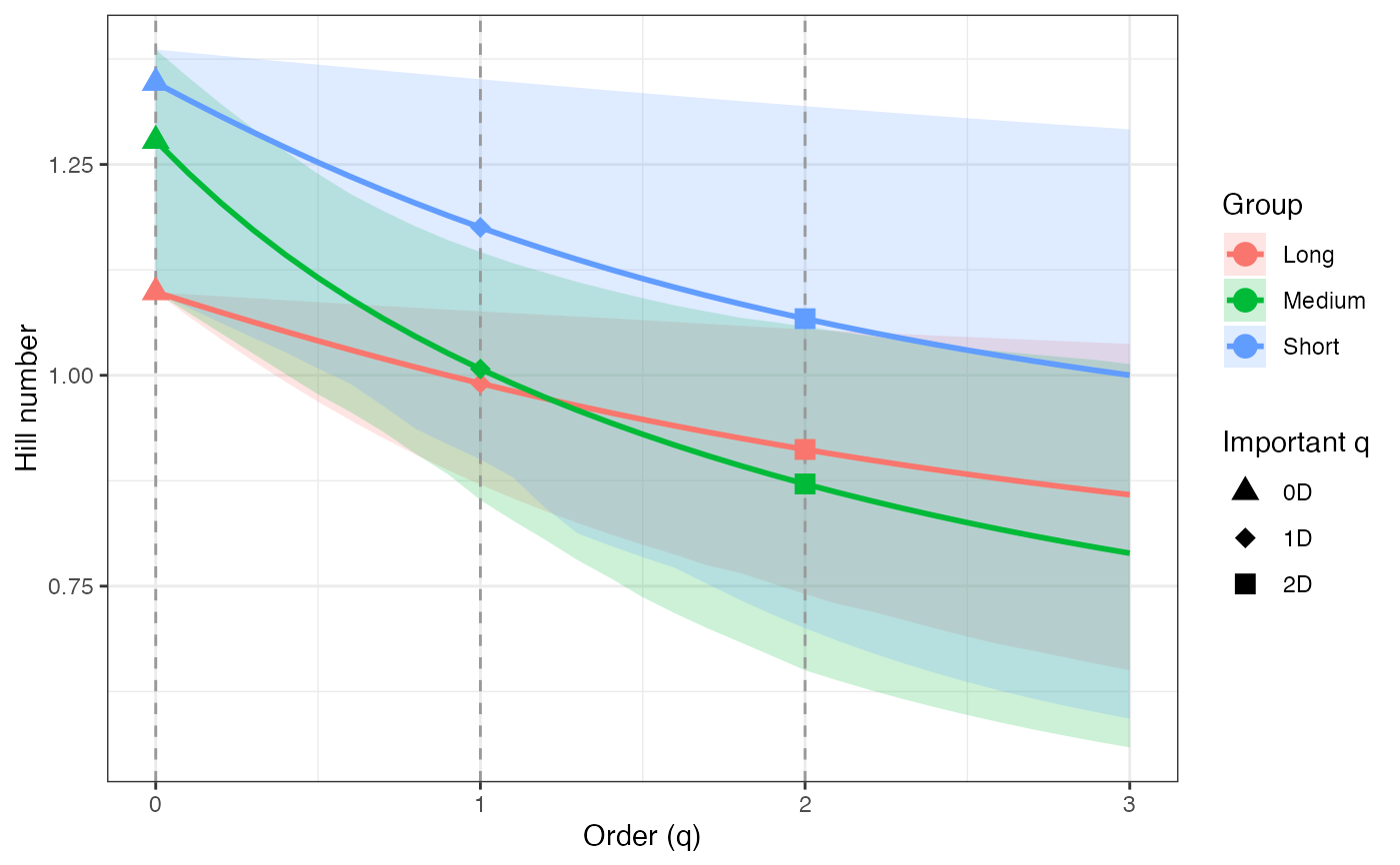
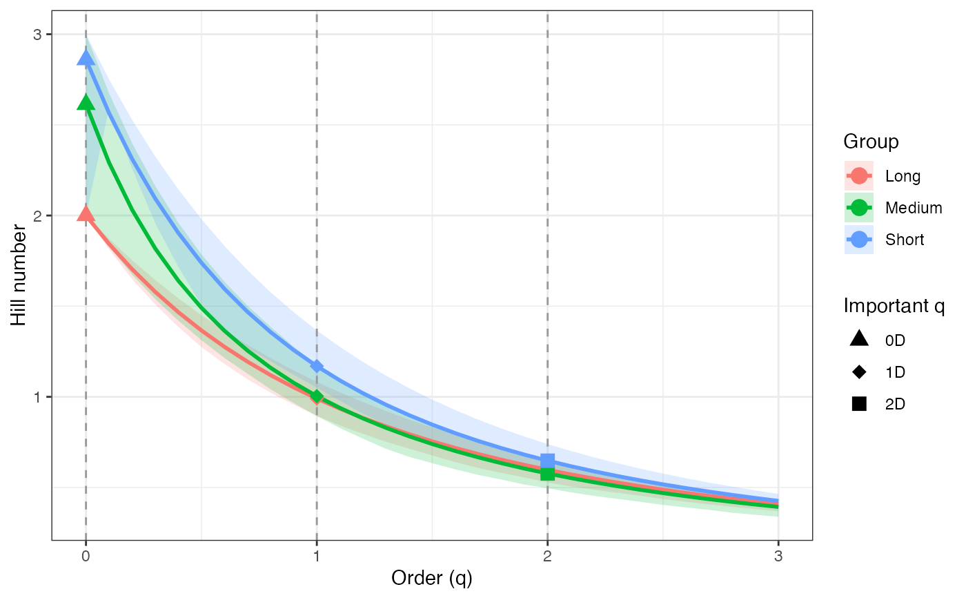
ggplot(tsallis_profile2_df, aes(x = q, y = mean,
color = group, fill = group)) +
geom_ribbon(aes(ymin = lower, ymax = upper), alpha = 0.2, color = NA) +
geom_line(linewidth = 1) +
geom_vline(xintercept = c(0, 1, 2), linetype = "dashed",
color = "grey60") +
geom_point(data = tsallis_points2_df, aes(shape = order_label),
size = 3, stroke = 1, inherit.aes = TRUE) +
scale_shape_manual(values = c(17, 18, 15), name = "Important q") +
labs(x = "Order (q)", y = "Hill number",
color = "Group", fill = "Group") +
theme_bw()
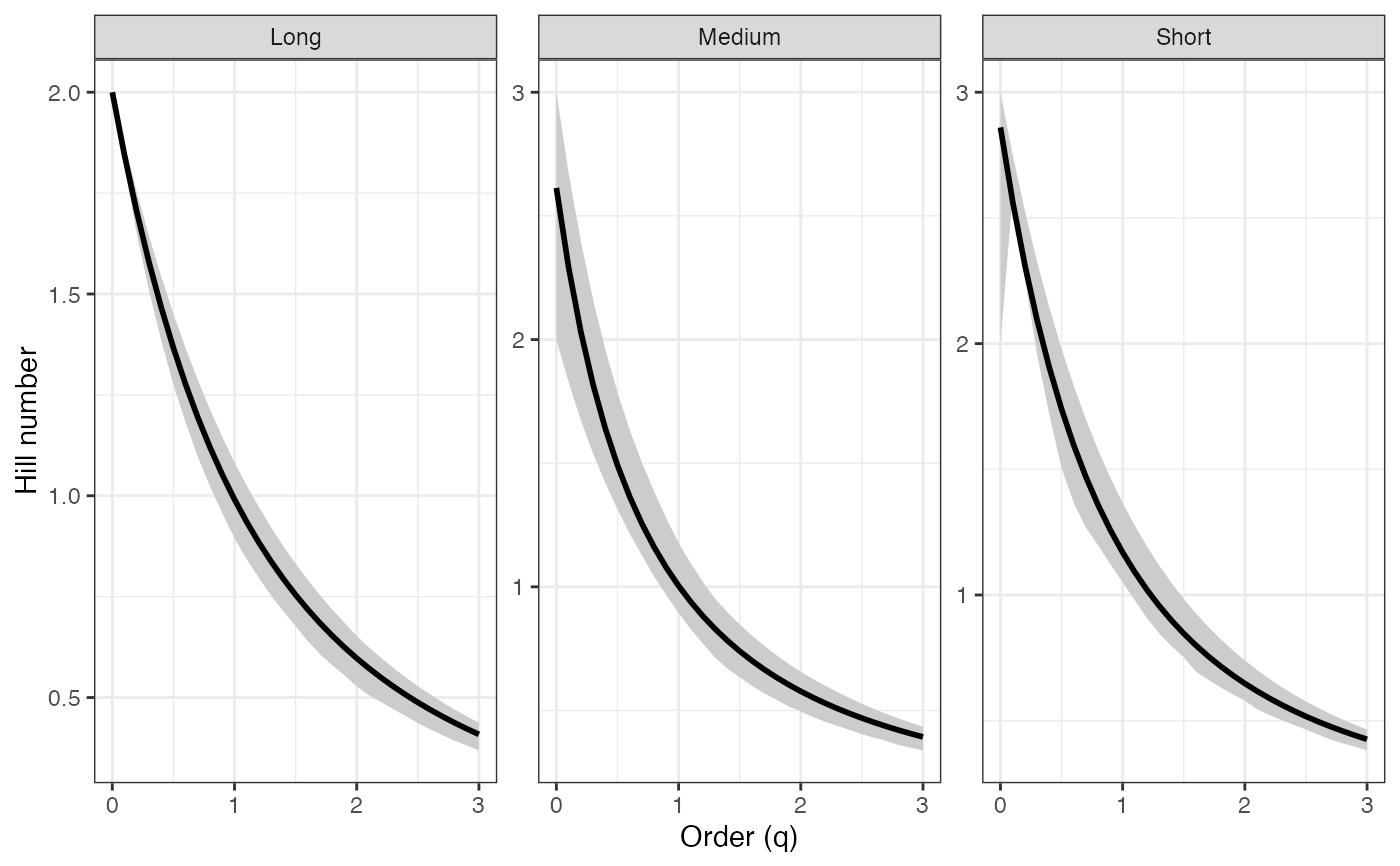
 ggplot(tsallis_profile2_df, aes(x = q, y = mean)) +
geom_ribbon(aes(ymin = lower, ymax = upper), fill = "grey80") +
geom_line(color = "black", linewidth = 1) +
facet_wrap(~ group, scales = "free_y") +
labs(x = "Order (q)", y = "Hill number") +
theme_bw()
ggplot(tsallis_profile2_df, aes(x = q, y = mean)) +
geom_ribbon(aes(ymin = lower, ymax = upper), fill = "grey80") +
geom_line(color = "black", linewidth = 1) +
facet_wrap(~ group, scales = "free_y") +
labs(x = "Order (q)", y = "Hill number") +
theme_bw()