Seed viability curve fitting to estimate multiple values of K_i and σ according to a grouping variable

Fit seed viability/survival curve to estimate multiple values of the seed lot constant (K_i) and the period to lose unit probit viability (σ) according to a grouping variable.

FitSigma.batch(data, group, ...)

Arguments

data	A data frame with the seed viability data recorded periodically. It should possess columns with data on Viability percentage (to be indicated by the argument viability.percent), Sample size (to be indicated by the argument samp.size), Storage period (to be indicated by the argument storage.period) and Grouping variable (to be indicated by the argument group).
group	The name of the column in data with grouping variable as a character string.
...	Arguments to be passed on to FitSigma.

Value

A list of class FitSigma.batch with the following components:

data

A data frame with the data used for computing the models.

models

A data frame with the group-wise values of model parameters, K_i and σ and the fit statistics.

See also

FitSigma

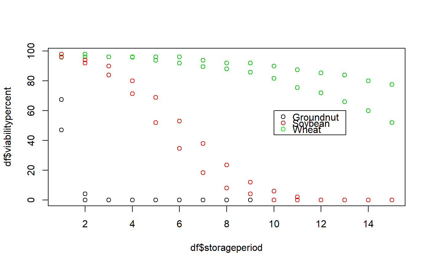
Examples

data(seedsurvival)
df <- seedsurvival[seedsurvival$moistruecontent == 7 &
                     seedsurvival$temperature == 25,
                   c("crop", "storageperiod", "rep",
                     "viabilitypercent", "sampsize")]

plot(df$storageperiod, df$viabilitypercent, col = df$crop)
legend(10, 60, legend=levels(df$crop),
       col = c("black", "red", "green"), pch = 1)

#----------------------------------------------------------------------------
# Generalised linear model with probit link function (without cv)
#----------------------------------------------------------------------------
model1a <- FitSigma.batch(data = df, group = "crop",
                          viability.percent = "viabilitypercent",
                          samp.size = "sampsize",
                          storage.period = "storageperiod",
                          generalised.model = TRUE)
#> WARNING: glm.fit: fitted probabilities numerically 0 or 1 occurred 
#> NA 
#> NA 
model1a
#> Generalised linear model with probit link function.
#>      group       Ki     sigma
#>  Groundnut 2.402050 0.4500519
#>    Soybean 2.373913 2.3620603
#>      Wheat 2.154888 8.7682357
#> 

#----------------------------------------------------------------------------
# Generalised linear model with probit link function (with cv)
#----------------------------------------------------------------------------
model1b <- FitSigma.batch(data = df, group = "crop",
                          viability.percent = "viabilitypercent",
                          samp.size = "sampsize",
                          storage.period = "storageperiod",
                          generalised.model = TRUE,
                          use.cv = TRUE, control.viability = 98)
#> WARNING: non-integer #successes in a binomial glm! 
#> WARNING: glm.fit: fitted probabilities numerically 0 or 1 occurred 
#> Warning: the condition has length > 1 and only the first element will be used
#> WARNING: non-integer #successes in a binomial glm! 
#> WARNING: non-integer #successes in a binomial glm! 
model1b
#> Generalised linear model with probit link function.
#> Control viability = 98%
#>      group       Ki     sigma
#>  Groundnut 2.453183 0.4457701
#>  Groundnut 2.453183 0.4457701
#>    Soybean 2.543327 2.2522451
#>      Wheat 2.501611 7.2669575
#> 
#>      group                                                            message
#>  Groundnut                 WARNING: non-integer #successes in a binomial glm!
#>  Groundnut WARNING: glm.fit: fitted probabilities numerically 0 or 1 occurred
#>    Soybean                 WARNING: non-integer #successes in a binomial glm!
#>      Wheat                 WARNING: non-integer #successes in a binomial glm!

#----------------------------------------------------------------------------
# Linear model after probit transformation (without cv)
#----------------------------------------------------------------------------
model2a <- FitSigma.batch(data = df, group = "crop",
                          viability.percent = "viabilitypercent",
                          samp.size = "sampsize",
                          storage.period = "storageperiod",
                          generalised.model = FALSE)
#> NA 
#> NA 
#> NA 
model2a
#> Linear model after probit transformation.
#>      group        Ki     sigma
#>  Groundnut -1.733721 12.772161
#>    Soybean  2.014134  2.810871
#>      Wheat  2.103905  9.393616
#> 

#----------------------------------------------------------------------------
# Linear model after probit transformation (with cv)
#----------------------------------------------------------------------------
model2b <- FitSigma.batch(data = df, group = "crop",
                          viability.percent = "viabilitypercent",
                          samp.size = "sampsize",
                          storage.period = "storageperiod",
                          generalised.model = FALSE,
                          use.cv = TRUE, control.viability = 98)
#> NA 
#> NA 
#> NA 
model2b
#> Linear model after probit transformation.
#> Control viability = 98%
#>      group        Ki     sigma
#>  Groundnut -1.769103 12.516718
#>    Soybean  2.055239  2.754653
#>      Wheat  2.146842  9.205744
#>