Plot the fitted seed viability curves from a <code>FitSigma.batch</code> object

plot.FitSigma.batch plots the group-wise fitted seed viability/survival curves from a FitSigma.batch object as an object of class ggplot.

# S3 method for FitSigma.batch
plot(x, limits = TRUE, grid = FALSE, ...)

Arguments

x	An object of class `FitSigma.batch` obtained as output from the `FitSigma.batch` function.
limits	logical. If `TRUE`, set the limits of y axis (viability percentage) between 0 and 100 in the viability curve plot. If `FALSE`, limits are set according to the data. Default is `TRUE`.
grid	logical. If `TRUE`, a symmetric matrix grid of plots is produced instead of a single plot with multiple curves. Default is `FALSE`.
...	Default plot arguments.

Value

The plot of the seed viability curves as an object of class ggplot.

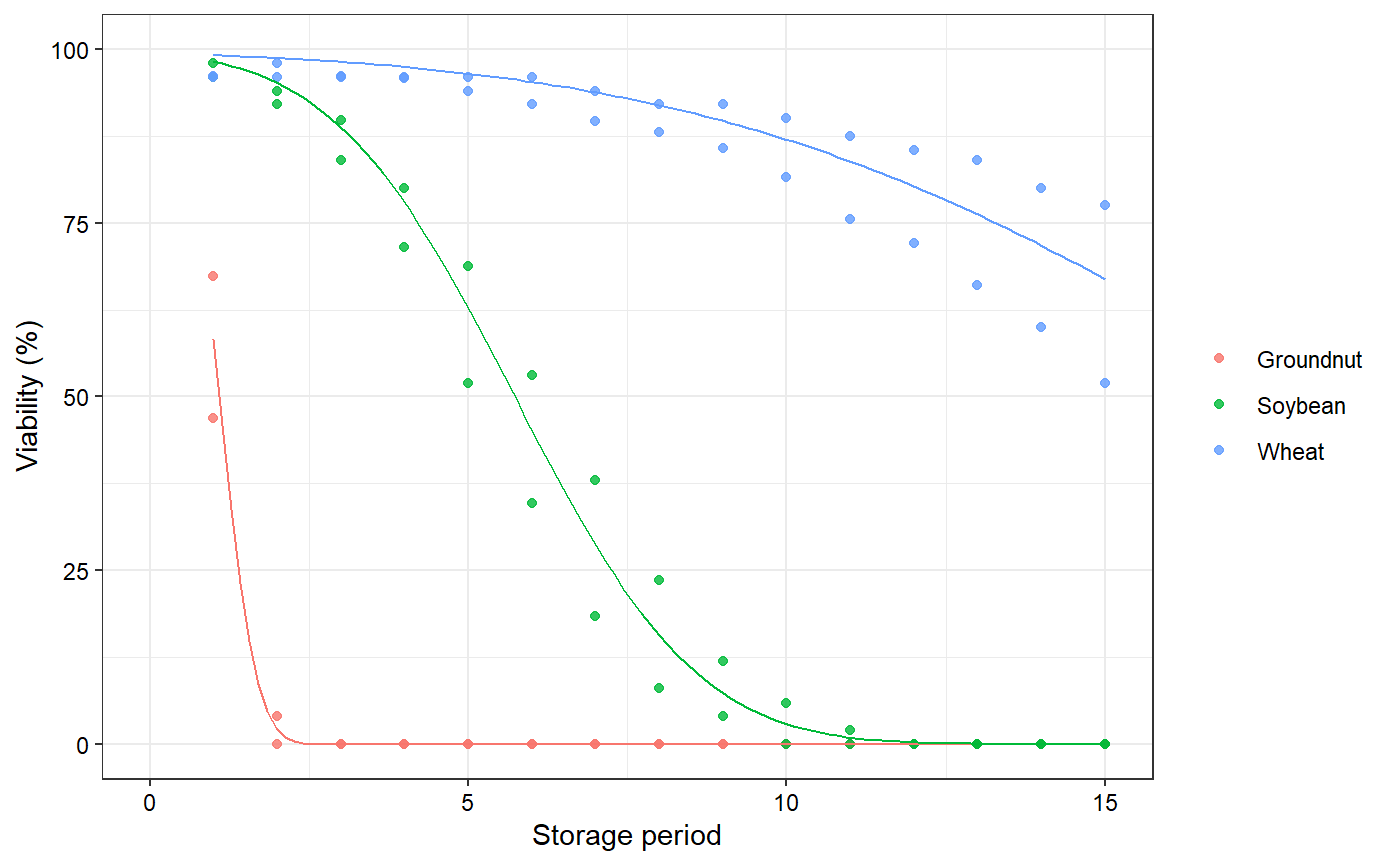
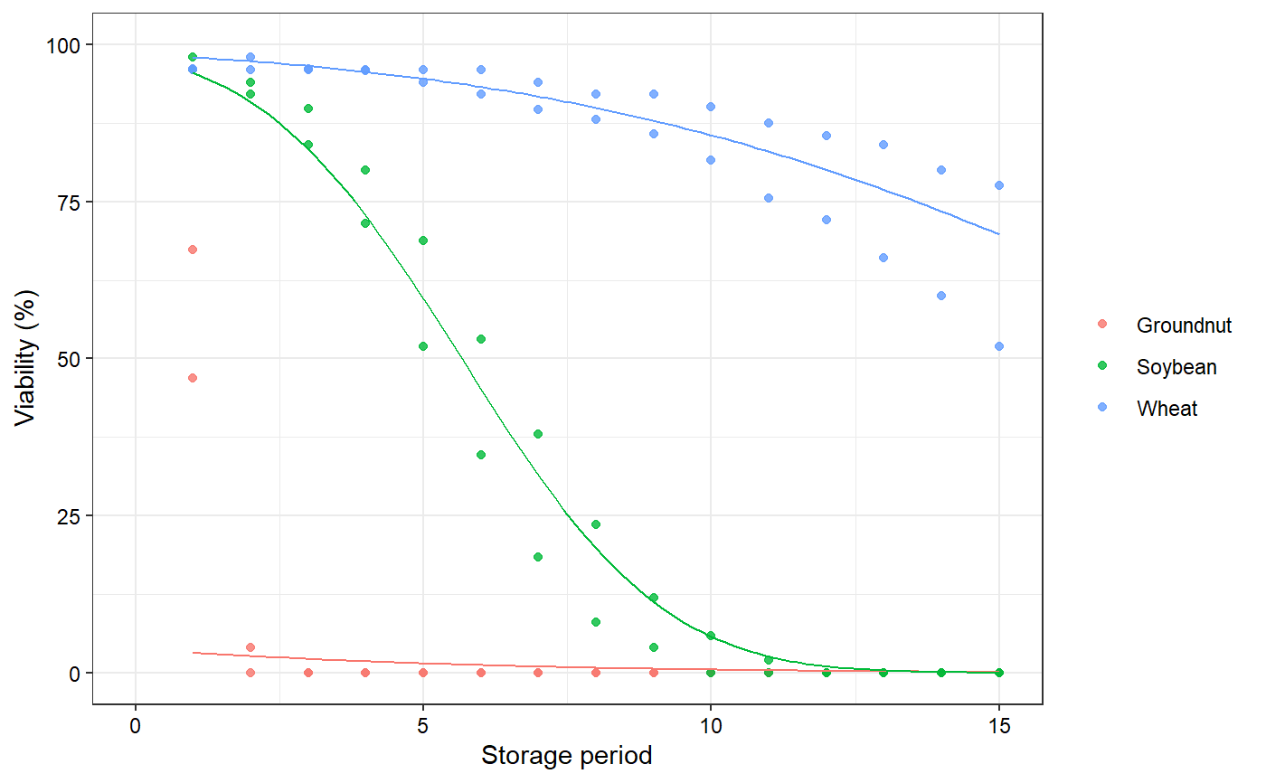
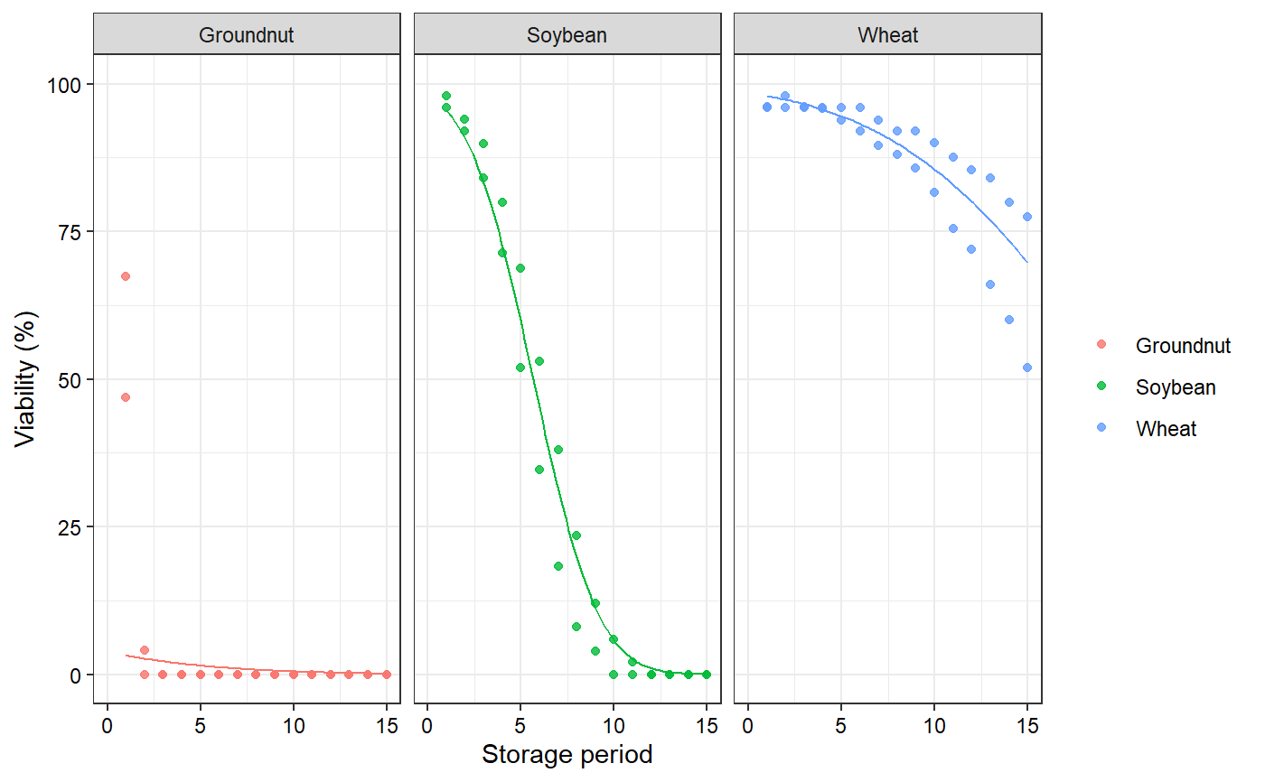
Examples


data(seedsurvival)
df <- seedsurvival[seedsurvival$moistruecontent == 7 &
                     seedsurvival$temperature == 25,
                   c("crop", "storageperiod", "rep",
                     "viabilitypercent", "sampsize")]

#----------------------------------------------------------------------------
# Generalised linear model with probit link function (without cv)
#----------------------------------------------------------------------------
model1a <- FitSigma.batch(data = df, group = "crop",
                          viability.percent = "viabilitypercent",
                          samp.size = "sampsize",
                          storage.period = "storageperiod",
                          generalised.model = TRUE)
#> WARNING: glm.fit: fitted probabilities numerically 0 or 1 occurred 
#> NA 
#> NA 
plot(model1a)
plot(model1a, grid = TRUE)

#----------------------------------------------------------------------------
# Generalised linear model with probit link function (with cv)
#----------------------------------------------------------------------------
model1b <- FitSigma.batch(data = df, group = "crop",
                          viability.percent = "viabilitypercent",
                          samp.size = "sampsize",
                          storage.period = "storageperiod",
                          generalised.model = TRUE,
                          use.cv = TRUE, control.viability = 98)
#> WARNING: non-integer #successes in a binomial glm! 
#> WARNING: glm.fit: fitted probabilities numerically 0 or 1 occurred 
#> Warning: the condition has length > 1 and only the first element will be used
#> WARNING: non-integer #successes in a binomial glm! 
#> WARNING: non-integer #successes in a binomial glm! 
plot(model1b)
#> Warning: the condition has length > 1 and only the first element will be used
#> Warning: longer object length is not a multiple of shorter object length
#> Warning: longer object length is not a multiple of shorter object length
plot(model1b, grid = TRUE)
#> Warning: the condition has length > 1 and only the first element will be used
#> Warning: longer object length is not a multiple of shorter object length
#> Warning: longer object length is not a multiple of shorter object length

#----------------------------------------------------------------------------
# Linear model after probit transformation (without cv)
#----------------------------------------------------------------------------
model2a <- FitSigma.batch(data = df, group = "crop",
                          viability.percent = "viabilitypercent",
                          samp.size = "sampsize",
                          storage.period = "storageperiod",
                          generalised.model = FALSE)
#> NA 
#> NA 
#> NA 
plot(model2a)
plot(model2a, grid = TRUE)

#----------------------------------------------------------------------------
# Linear model after probit transformation (with cv)
#----------------------------------------------------------------------------
model2b <- FitSigma.batch(data = df, group = "crop",
                          viability.percent = "viabilitypercent",
                          samp.size = "sampsize",
                          storage.period = "storageperiod",
                          generalised.model = FALSE,
                          use.cv = TRUE, control.viability = 98)
#> NA 
#> NA 
#> NA 
plot(model2b)
plot(model2b, grid = TRUE)