Plot the fitted seed viability curve from a FitSigma object

plot.FitSigma plots the fitted seed viability/survival curve from a FitSigma object as an object of class ggplot.

# S3 method for FitSigma
plot(x, limits = TRUE, annotate = TRUE, ...)

Arguments

x	An object of class FitSigma obtained as output from the FitSigma function.
limits	logical. If TRUE, set the limits of y axis (viability percentage) between 0 and 100 in the viability curve plot. If FALSE, limits are set according to the data. Default is TRUE.
annotate	logical. If TRUE, Ki and σ values are annotated on the plot. Default is TRUE.
...	Default plot arguments.

Value

The plot of the seed viability curve as an object of class ggplot.

See also

FitSigma

Examples

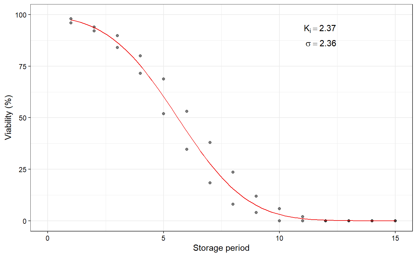
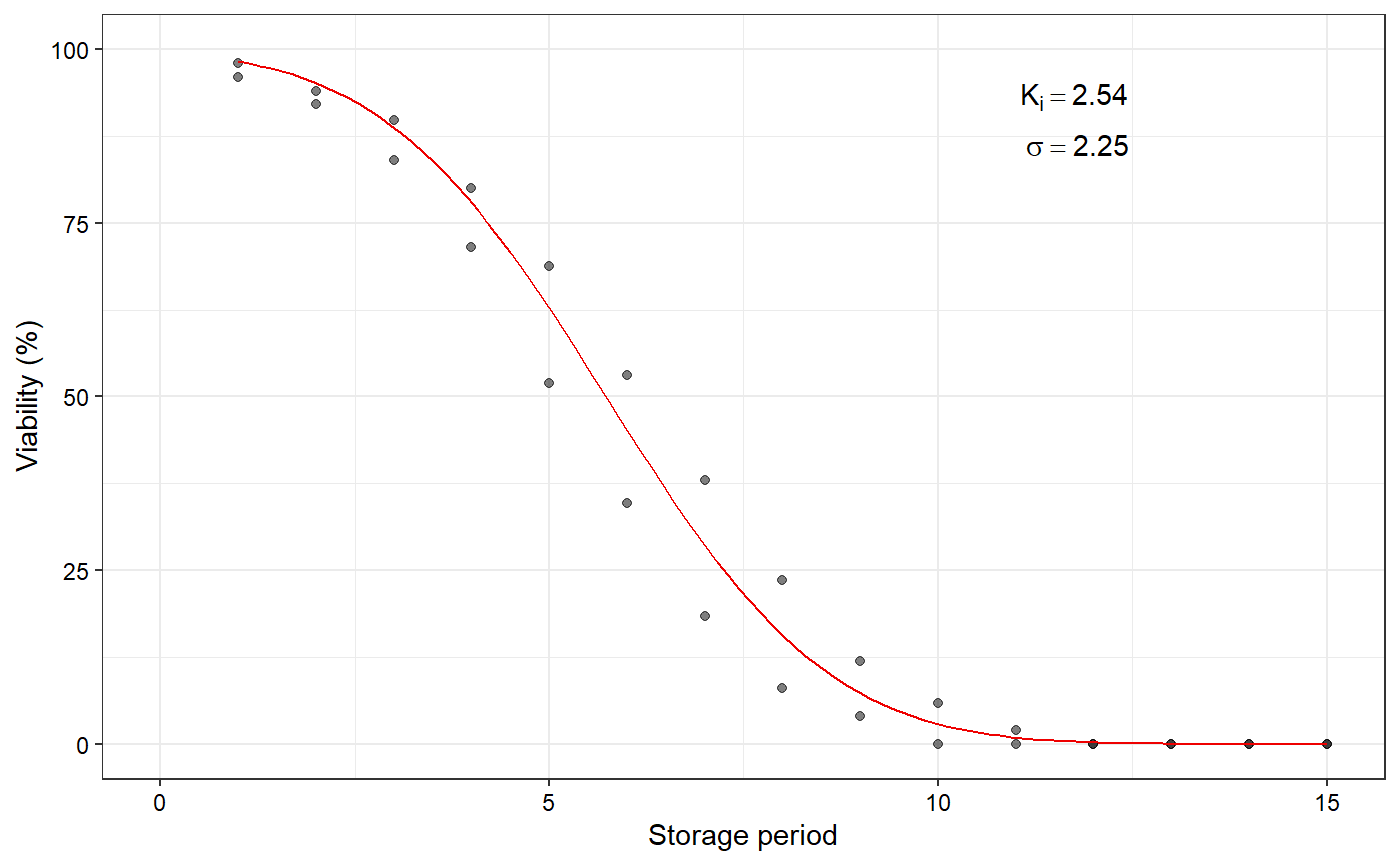
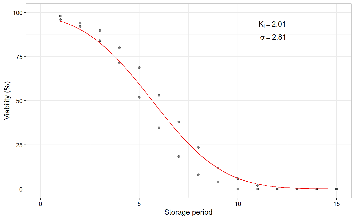
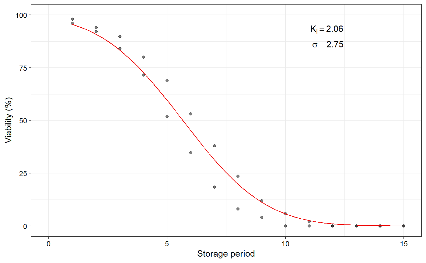
data(seedsurvival)
df <- seedsurvival[seedsurvival$crop == "Soybean" &
                     seedsurvival$moistruecontent == 7 &
                     seedsurvival$temperature == 25,
                   c("storageperiod", "rep",
                     "viabilitypercent", "sampsize")]

#----------------------------------------------------------------------------
# Generalised linear model with probit link function (without cv)
#----------------------------------------------------------------------------
model1a <- FitSigma(data = df, viability.percent = "viabilitypercent",
                   samp.size = "sampsize", storage.period = "storageperiod",
                   generalised.model = TRUE)
#> NA 
plot(model1a)

#----------------------------------------------------------------------------
# Generalised linear model with probit link function (with cv)
#----------------------------------------------------------------------------
model1b <- FitSigma(data = df, viability.percent = "viabilitypercent",
                   samp.size = "sampsize", storage.period = "storageperiod",
                   generalised.model = TRUE,
                   use.cv = TRUE, control.viability = 98)
#> WARNING: non-integer #successes in a binomial glm! 
plot(model1b)

#----------------------------------------------------------------------------
# Linear model after probit transformation (without cv)
#----------------------------------------------------------------------------
model2a <- FitSigma(data = df, viability.percent = "viabilitypercent",
                   samp.size = "sampsize", storage.period = "storageperiod",
                   generalised.model = FALSE)
#> NA 
plot(model2a)

#----------------------------------------------------------------------------
# Linear model after probit transformation (with cv)
#----------------------------------------------------------------------------
model2b <- FitSigma(data = df, viability.percent = "viabilitypercent",
                   samp.size = "sampsize", storage.period = "storageperiod",
                   generalised.model = FALSE,
                   use.cv = TRUE, control.viability = 98)
#> NA 
plot(model2b)