An example germplasm characterisation data of a core collection generated
from 1591 accessions of IITA Cassava collection
(International Institute of Tropical Agriculture et al. 2019)
using 10 quantitative and 48 qualitative trait data with CoreHunter3
(corehunter). The core set was generated using
distance based measures giving equal weightage to Average
entry-to-nearest-entry distance (EN) and Average accession-to-nearest-entry
distance (AN). Includes data on 26 descriptors for 168 (10 % of
cassava_EC) accessions. It is used to demonstrate
the various functions of EvaluateCore package.
Format
A data frame with 58 columns:
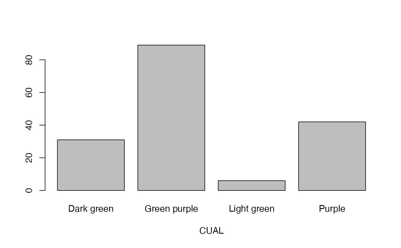
- CUAL
Colour of unexpanded apical leaves
- LNGS
Length of stipules
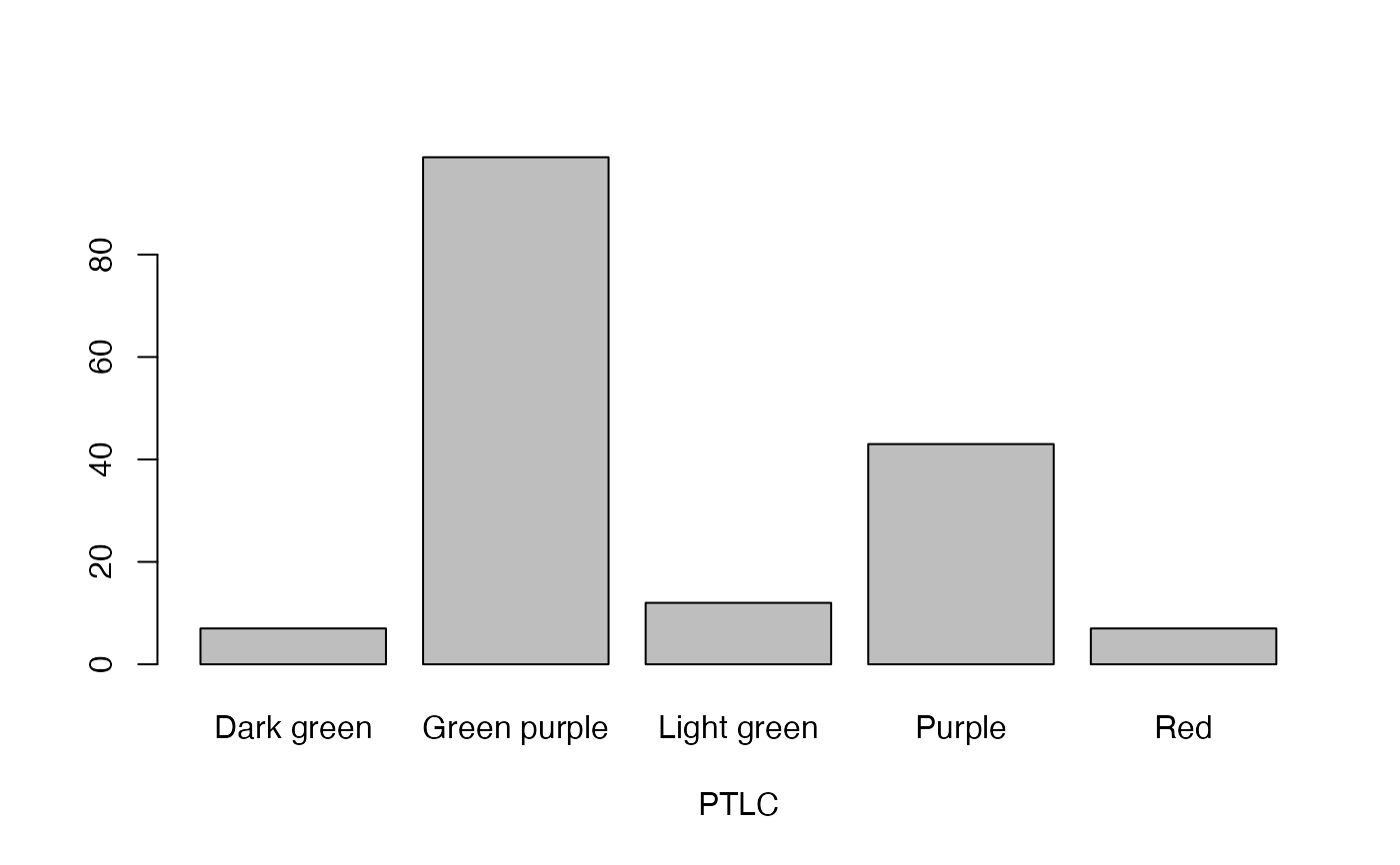
- PTLC
Petiole colour
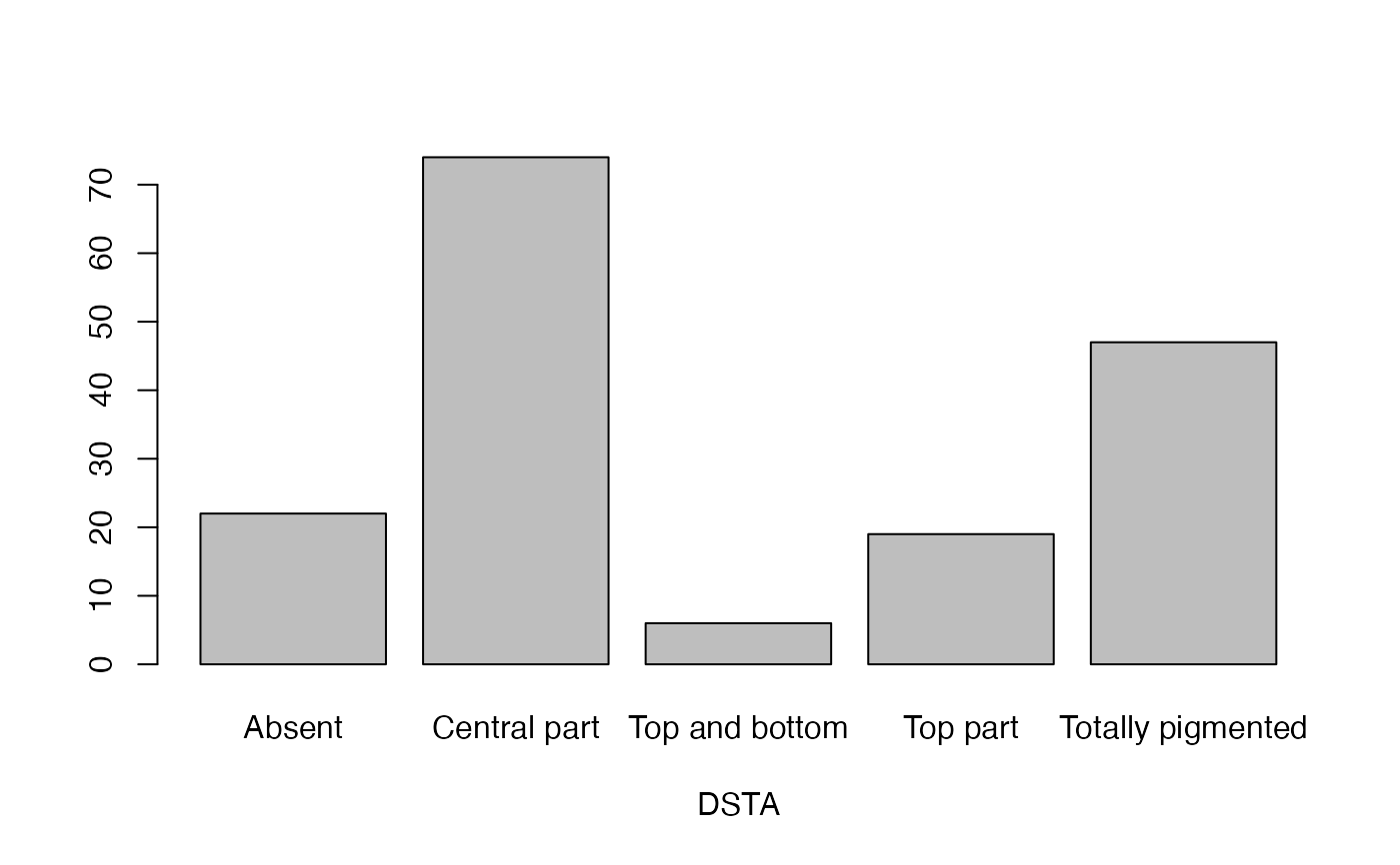
- DSTA
Distribution of anthocyanin
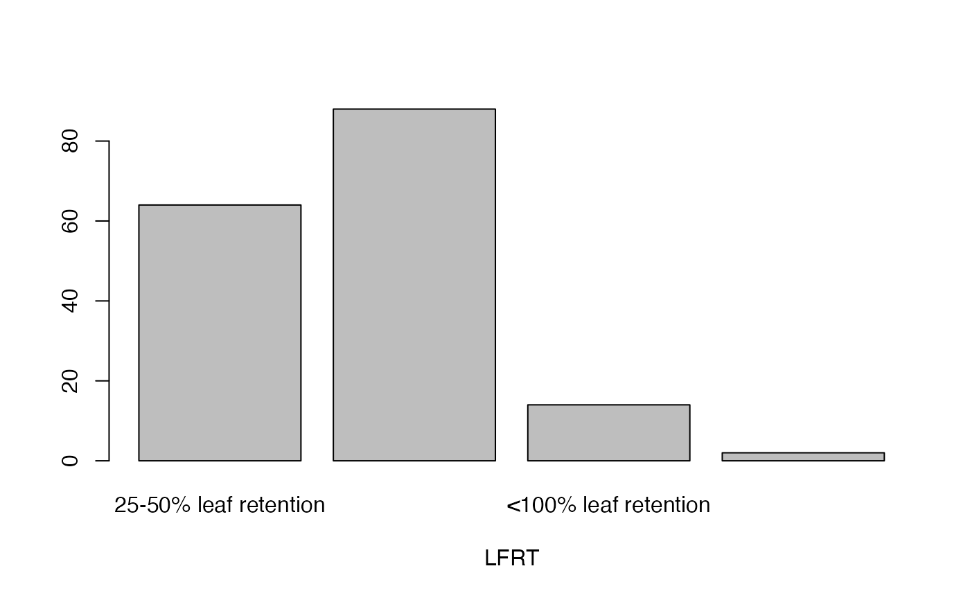
- LFRT
Leaf retention
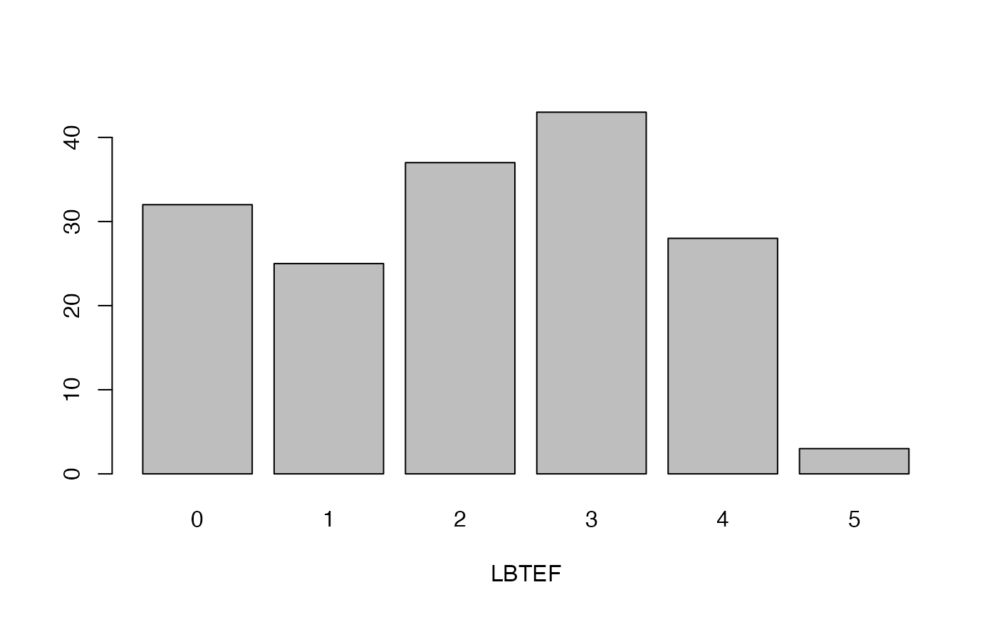
- LBTEF
Level of branching at the end of flowering
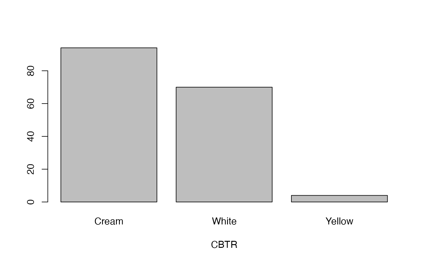
- CBTR
Colour of boiled tuberous root
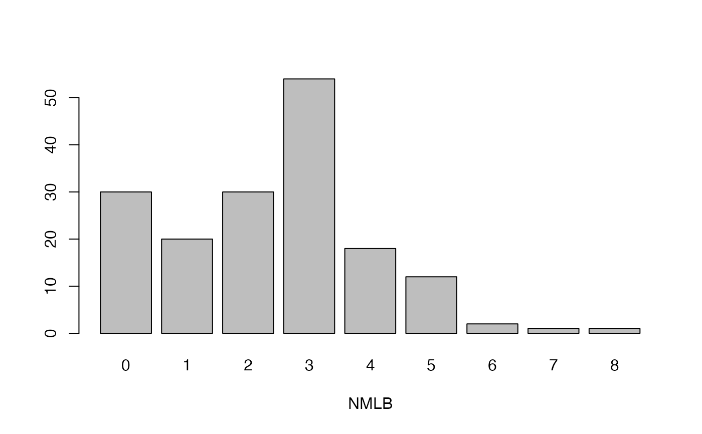
- NMLB
Number of levels of branching
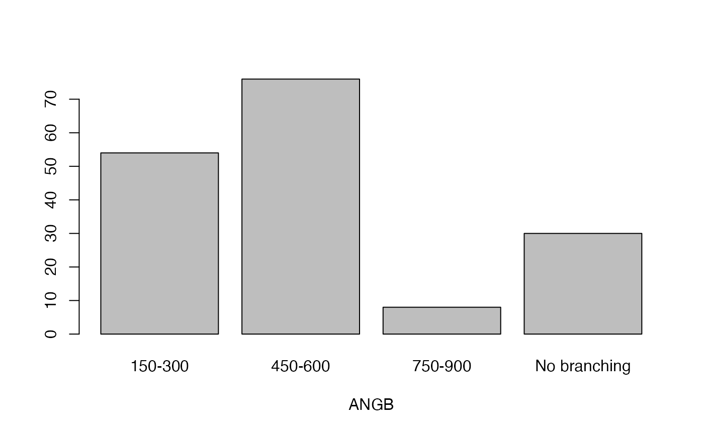
- ANGB
Angle of branching
- CUAL9M
Colours of unexpanded apical leaves at 9 months
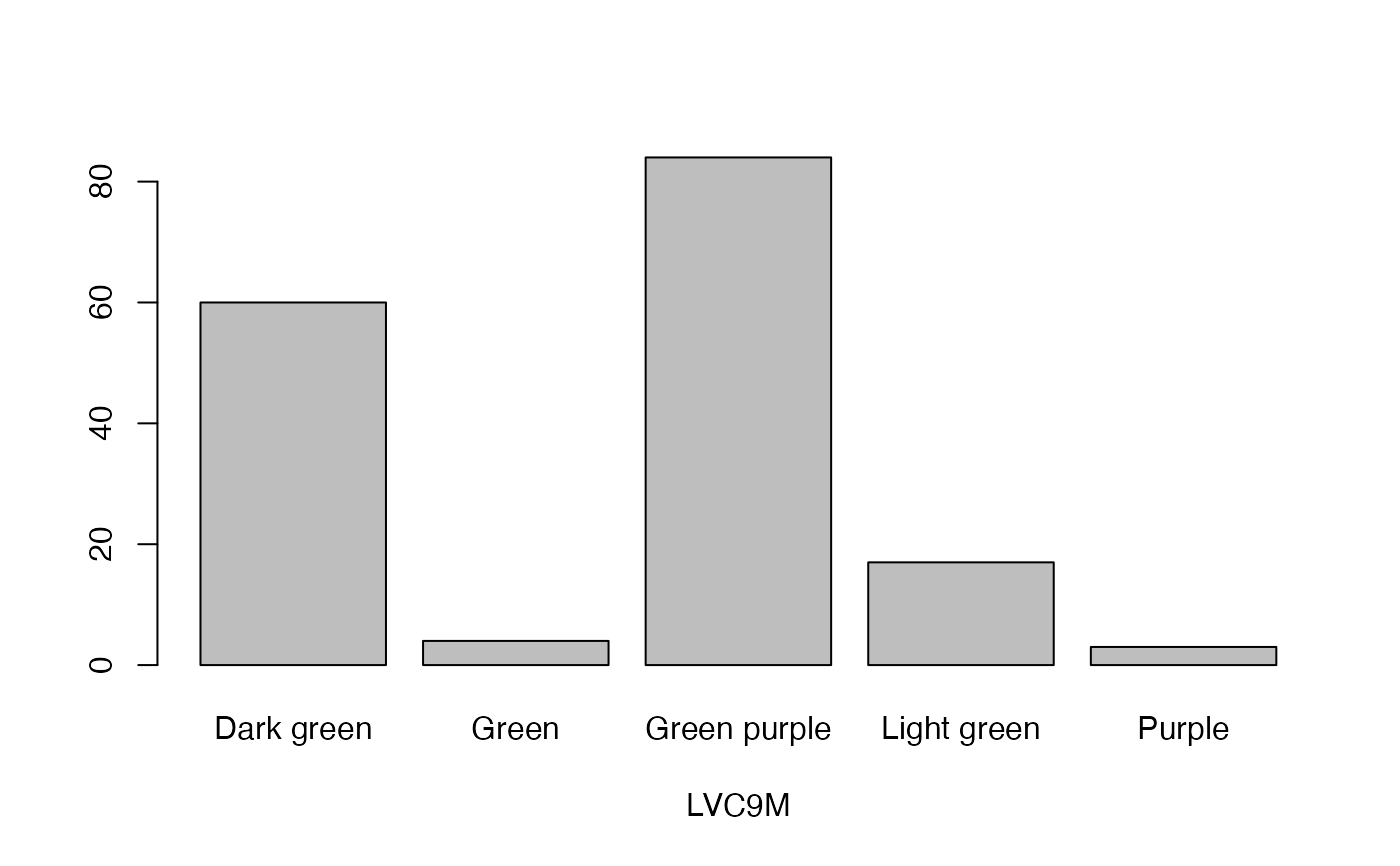
- LVC9M
Leaf vein colour at 9 months
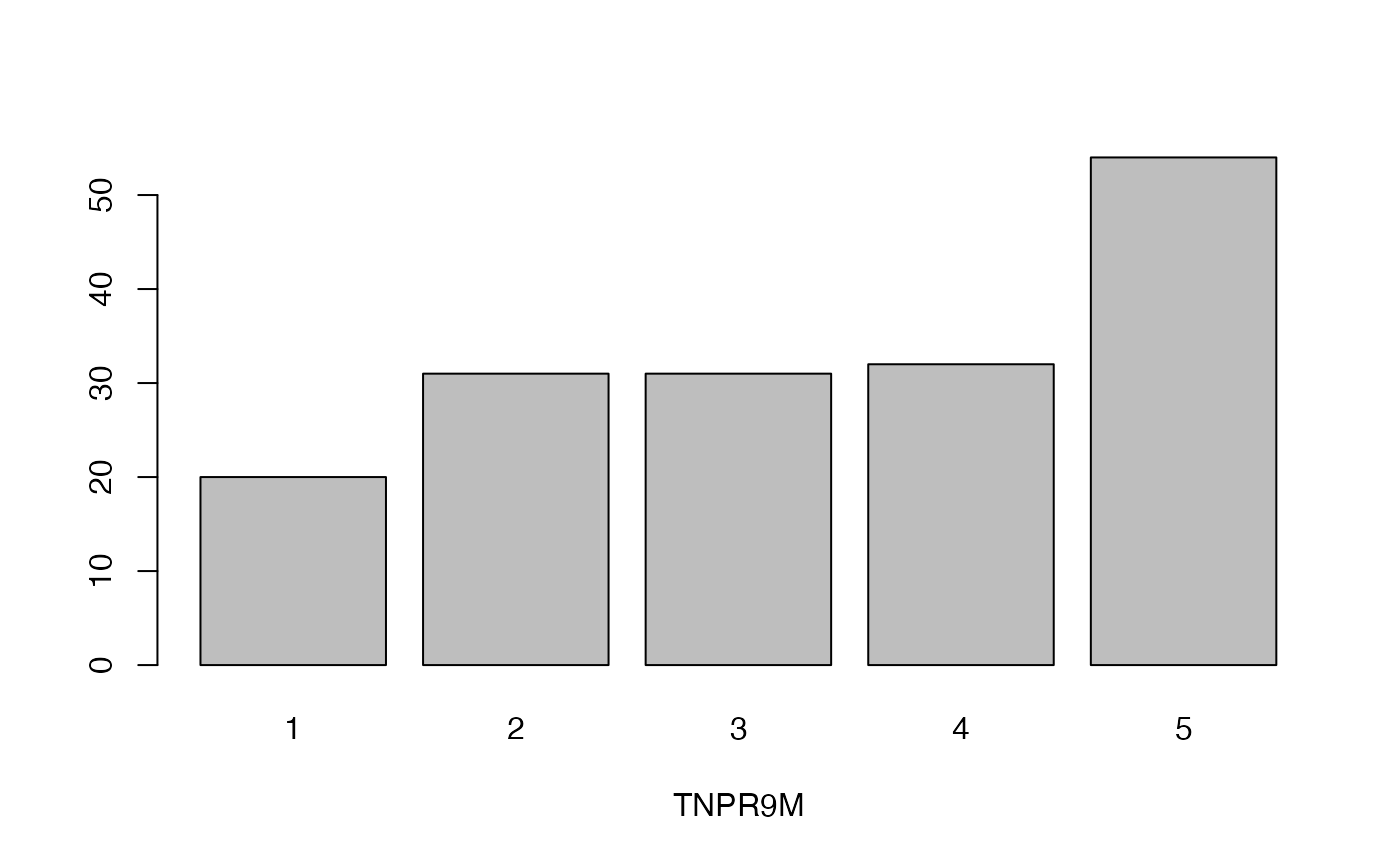
- TNPR9M
Total number of plants remaining per accession at 9 months
- PL9M
Petiole length at 9 months
- STRP
Storage root peduncle
- STRC
Storage root constrictions
- PSTR
Position of root
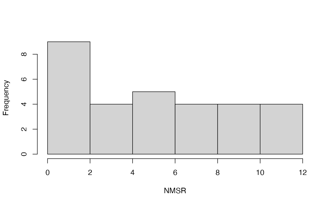
- NMSR
Number of storage root per plant
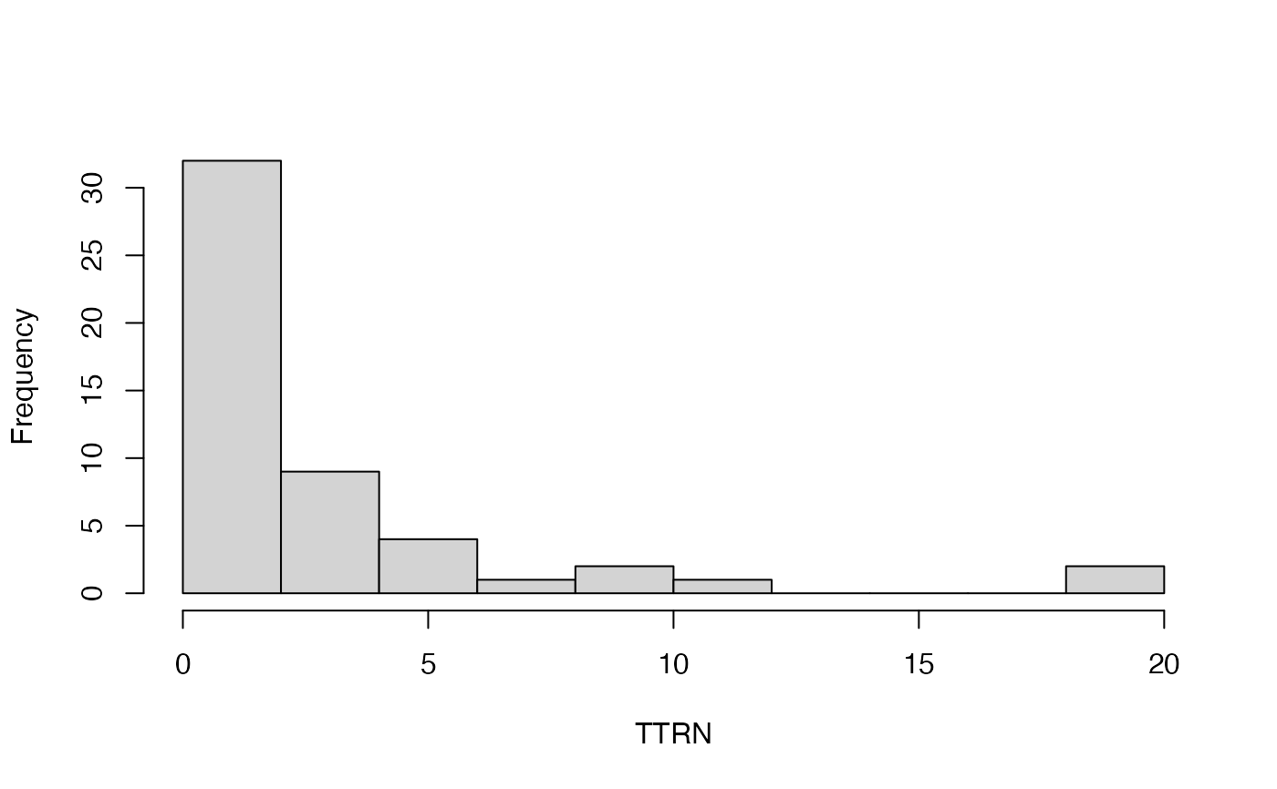
- TTRN
Total root number per plant
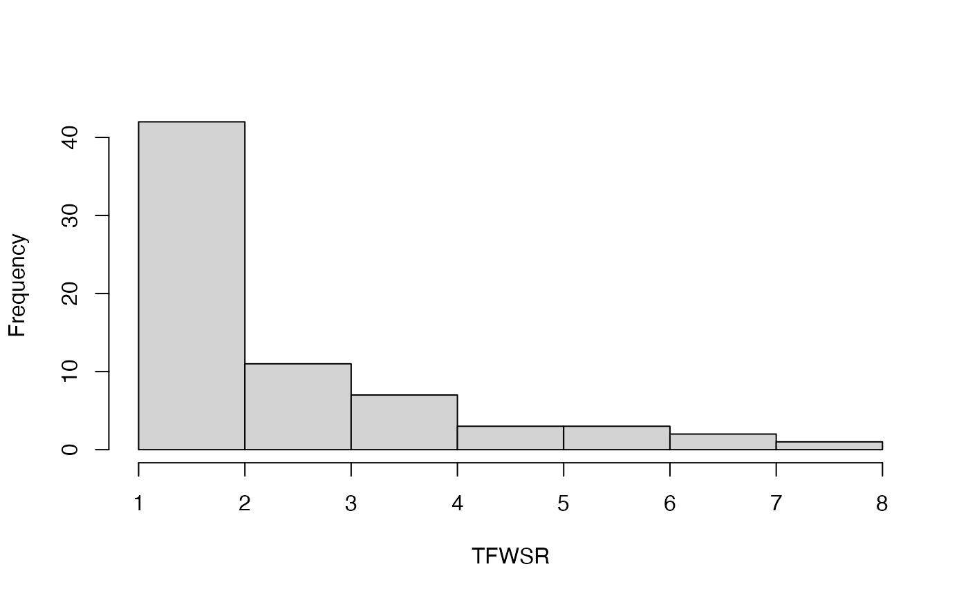
- TFWSR
Total fresh weight of storage root per plant
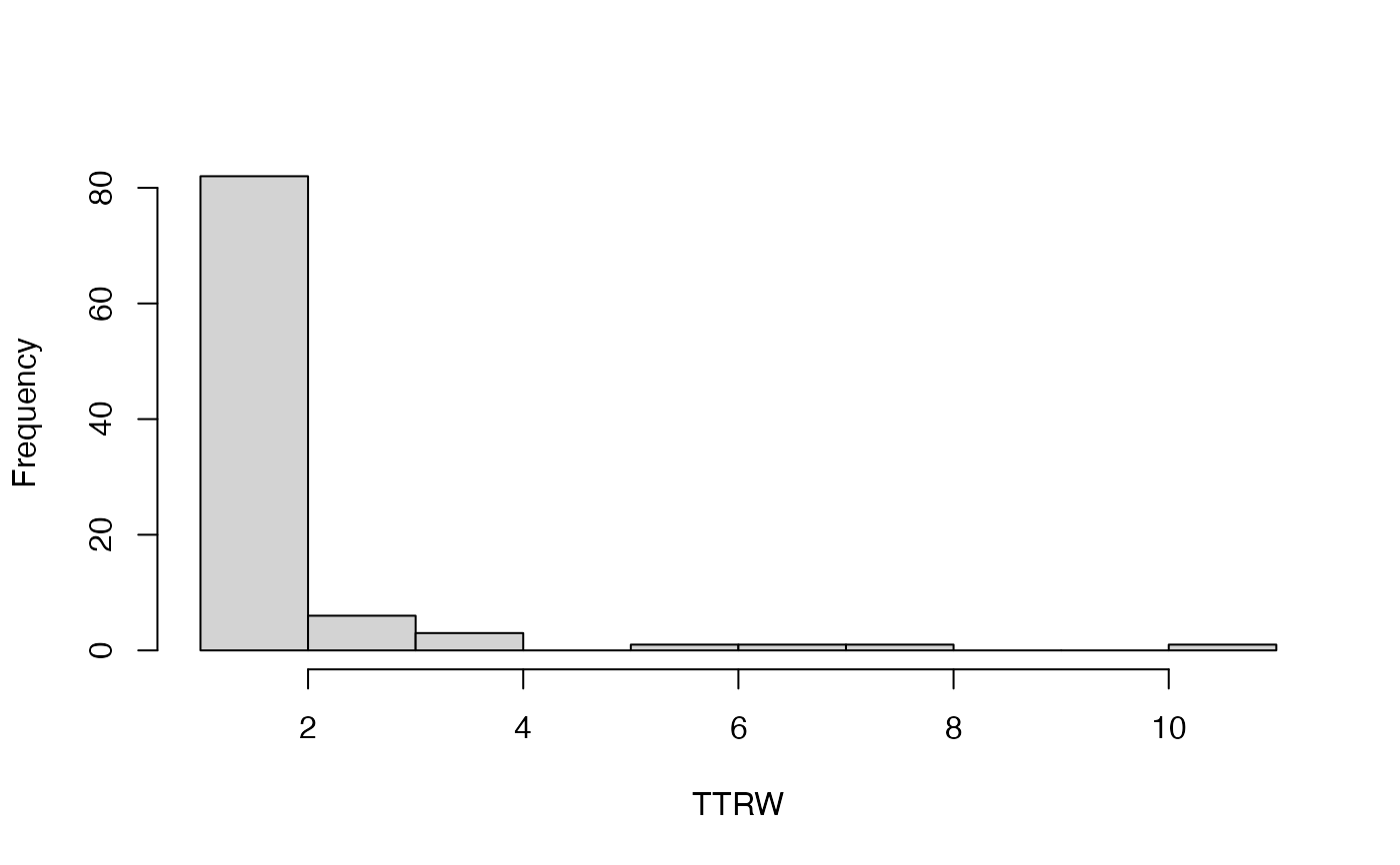
- TTRW
Total root weight per plant
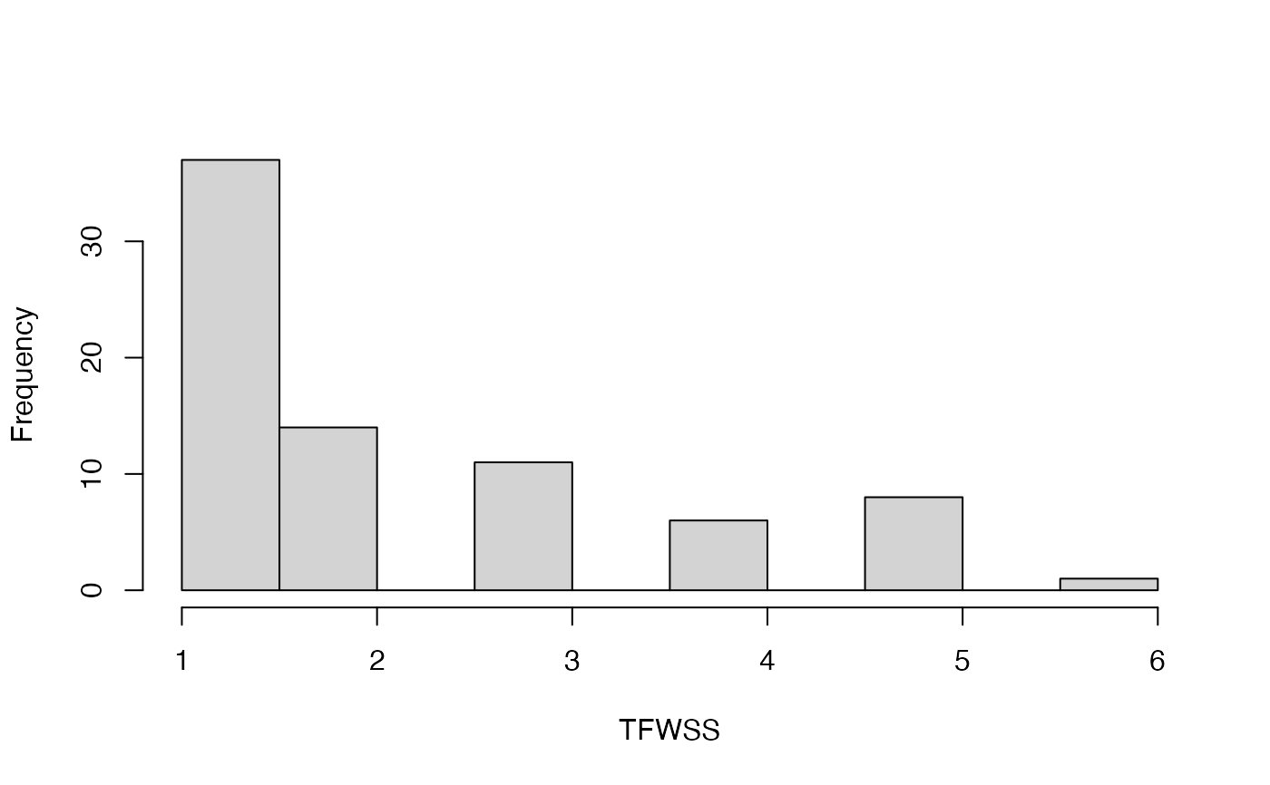
- TFWSS
Total fresh weight of storage shoot per plant
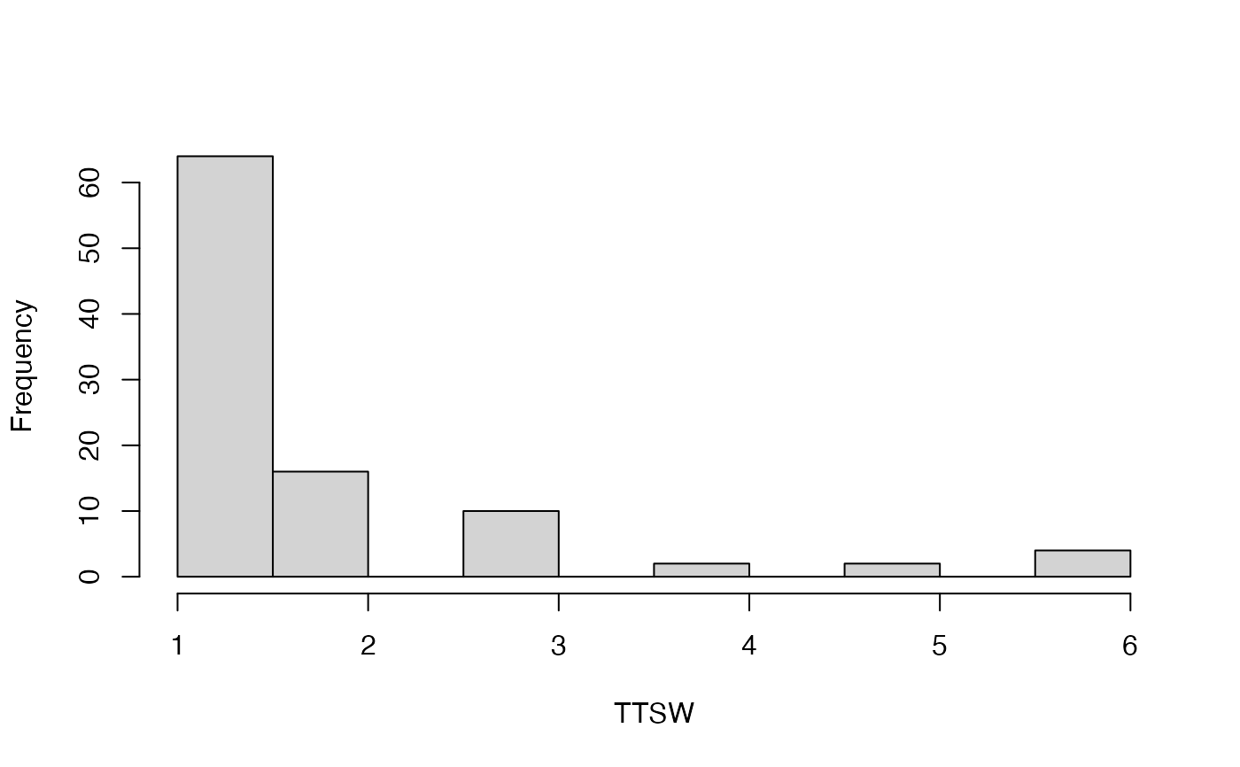
- TTSW
Total shoot weight per plant
- TTPW
Total plant weight
- AVPW
Average plant weight
- ARSR
Amount of rotted storage root per plant
- SRDM
Storage root dry matter
Details
Further details on how the example dataset was built from the original data is available online.
References
International Institute of Tropical Agriculture, Benjamin F, Marimagne T (2019). “Cassava morphological characterization. Version 2018.1.”
Examples
data(cassava_CC)
summary(cassava_CC)
#> CUAL LNGS PTLC DSTA
#> Length :168 Length :168 Length :168 Length :168
#> N.unique : 4 N.unique : 3 N.unique : 5 N.unique : 5
#> N.blank : 0 N.blank : 0 N.blank : 0 N.blank : 0
#> Min.nchar: 6 Min.nchar: 4 Min.nchar: 3 Min.nchar: 6
#> Max.nchar: 12 Max.nchar: 6 Max.nchar: 12 Max.nchar: 17
#>
#> LFRT LBTEF CBTR NMLB
#> Length :168 Length :168 Length :168 Length :168
#> N.unique : 4 N.unique : 6 N.unique : 3 N.unique : 9
#> N.blank : 0 N.blank : 0 N.blank : 0 N.blank : 0
#> Min.nchar: 19 Min.nchar: 1 Min.nchar: 5 Min.nchar: 1
#> Max.nchar: 21 Max.nchar: 1 Max.nchar: 6 Max.nchar: 1
#>
#> ANGB CUAL9M LVC9M TNPR9M
#> Length :168 Length :168 Length :168 Length :168
#> N.unique : 4 N.unique : 5 N.unique : 5 N.unique : 5
#> N.blank : 0 N.blank : 0 N.blank : 0 N.blank : 0
#> Min.nchar: 7 Min.nchar: 5 Min.nchar: 5 Min.nchar: 1
#> Max.nchar: 12 Max.nchar: 12 Max.nchar: 12 Max.nchar: 1
#>
#> PL9M STRP STRC PSTR
#> Length :168 Length :168 Length :168 Length :168
#> N.unique : 2 N.unique : 4 N.unique : 2 N.unique : 2
#> N.blank : 0 N.blank : 0 N.blank : 0 N.blank : 0
#> Min.nchar: 14 Min.nchar: 4 Min.nchar: 6 Min.nchar: 9
#> Max.nchar: 16 Max.nchar: 12 Max.nchar: 7 Max.nchar: 25
#>
#> NMSR TTRN TFWSR TTRW
#> Min. : 1.00 Min. : 0.250 Min. : 0.200 Min. : 0.1000
#> 1st Qu.: 5.00 1st Qu.: 2.333 1st Qu.: 2.400 1st Qu.: 0.9333
#> Median : 9.00 Median : 3.500 Median : 4.300 Median : 1.5800
#> Mean :10.89 Mean : 3.931 Mean : 6.348 Mean : 2.6178
#> 3rd Qu.:14.25 3rd Qu.: 5.000 3rd Qu.: 7.950 3rd Qu.: 3.2000
#> Max. :55.00 Max. :13.750 Max. :38.000 Max. :20.2000
#> TFWSS TTSW TTPW AVPW
#> Min. : 0.200 Min. : 0.100 Min. : 0.40 Min. : 0.200
#> 1st Qu.: 2.700 1st Qu.: 1.113 1st Qu.: 5.35 1st Qu.: 2.190
#> Median : 5.400 Median : 2.058 Median :10.40 Median : 3.600
#> Mean : 7.748 Mean : 3.069 Mean :14.10 Mean : 5.687
#> 3rd Qu.:11.000 3rd Qu.: 3.950 3rd Qu.:19.00 3rd Qu.: 7.300
#> Max. :42.000 Max. :22.000 Max. :80.00 Max. :33.000
#> ARSR SRDM
#> Min. :0.000 Min. :21.90
#> 1st Qu.:0.000 1st Qu.:35.60
#> Median :1.000 Median :38.15
#> Mean :1.702 Mean :37.73
#> 3rd Qu.:3.000 3rd Qu.:40.23
#> Max. :8.000 Max. :48.10
quant <- c("NMSR", "TTRN", "TFWSR", "TTRW", "TFWSS", "TTSW", "TTPW", "AVPW",
"ARSR", "SRDM")
qual <- c("CUAL", "LNGS", "PTLC", "DSTA", "LFRT", "LBTEF", "CBTR", "NMLB",
"ANGB", "CUAL9M", "LVC9M", "TNPR9M", "PL9M", "STRP", "STRC",
"PSTR")
lapply(seq_along(cassava_CC[, qual]),
function(i) barplot(table(cassava_CC[, qual][, i]),
xlab = names(cassava_CC[, qual])[i]))


 #> [[1]]
#> [,1]
#> [1,] 0.7
#> [2,] 1.9
#> [3,] 3.1
#> [4,] 4.3
#>
#> [[2]]
#> [,1]
#> [1,] 0.7
#> [2,] 1.9
#> [3,] 3.1
#>
#> [[3]]
#> [,1]
#> [1,] 0.7
#> [2,] 1.9
#> [3,] 3.1
#> [4,] 4.3
#> [5,] 5.5
#>
#> [[4]]
#> [,1]
#> [1,] 0.7
#> [2,] 1.9
#> [3,] 3.1
#> [4,] 4.3
#> [5,] 5.5
#>
#> [[5]]
#> [,1]
#> [1,] 0.7
#> [2,] 1.9
#> [3,] 3.1
#> [4,] 4.3
#>
#> [[6]]
#> [,1]
#> [1,] 0.7
#> [2,] 1.9
#> [3,] 3.1
#> [4,] 4.3
#> [5,] 5.5
#> [6,] 6.7
#>
#> [[7]]
#> [,1]
#> [1,] 0.7
#> [2,] 1.9
#> [3,] 3.1
#>
#> [[8]]
#> [,1]
#> [1,] 0.7
#> [2,] 1.9
#> [3,] 3.1
#> [4,] 4.3
#> [5,] 5.5
#> [6,] 6.7
#> [7,] 7.9
#> [8,] 9.1
#> [9,] 10.3
#>
#> [[9]]
#> [,1]
#> [1,] 0.7
#> [2,] 1.9
#> [3,] 3.1
#> [4,] 4.3
#>
#> [[10]]
#> [,1]
#> [1,] 0.7
#> [2,] 1.9
#> [3,] 3.1
#> [4,] 4.3
#> [5,] 5.5
#>
#> [[11]]
#> [,1]
#> [1,] 0.7
#> [2,] 1.9
#> [3,] 3.1
#> [4,] 4.3
#> [5,] 5.5
#>
#> [[12]]
#> [,1]
#> [1,] 0.7
#> [2,] 1.9
#> [3,] 3.1
#> [4,] 4.3
#> [5,] 5.5
#>
#> [[13]]
#> [,1]
#> [1,] 0.7
#> [2,] 1.9
#>
#> [[14]]
#> [,1]
#> [1,] 0.7
#> [2,] 1.9
#> [3,] 3.1
#> [4,] 4.3
#>
#> [[15]]
#> [,1]
#> [1,] 0.7
#> [2,] 1.9
#>
#> [[16]]
#> [,1]
#> [1,] 0.7
#> [2,] 1.9
#>
lapply(seq_along(cassava_CC[, quant]),
function(i) hist(table(cassava_CC[, quant][, i]),
xlab = names(cassava_CC[, quant])[i],
main = ""))
#> [[1]]
#> [,1]
#> [1,] 0.7
#> [2,] 1.9
#> [3,] 3.1
#> [4,] 4.3
#>
#> [[2]]
#> [,1]
#> [1,] 0.7
#> [2,] 1.9
#> [3,] 3.1
#>
#> [[3]]
#> [,1]
#> [1,] 0.7
#> [2,] 1.9
#> [3,] 3.1
#> [4,] 4.3
#> [5,] 5.5
#>
#> [[4]]
#> [,1]
#> [1,] 0.7
#> [2,] 1.9
#> [3,] 3.1
#> [4,] 4.3
#> [5,] 5.5
#>
#> [[5]]
#> [,1]
#> [1,] 0.7
#> [2,] 1.9
#> [3,] 3.1
#> [4,] 4.3
#>
#> [[6]]
#> [,1]
#> [1,] 0.7
#> [2,] 1.9
#> [3,] 3.1
#> [4,] 4.3
#> [5,] 5.5
#> [6,] 6.7
#>
#> [[7]]
#> [,1]
#> [1,] 0.7
#> [2,] 1.9
#> [3,] 3.1
#>
#> [[8]]
#> [,1]
#> [1,] 0.7
#> [2,] 1.9
#> [3,] 3.1
#> [4,] 4.3
#> [5,] 5.5
#> [6,] 6.7
#> [7,] 7.9
#> [8,] 9.1
#> [9,] 10.3
#>
#> [[9]]
#> [,1]
#> [1,] 0.7
#> [2,] 1.9
#> [3,] 3.1
#> [4,] 4.3
#>
#> [[10]]
#> [,1]
#> [1,] 0.7
#> [2,] 1.9
#> [3,] 3.1
#> [4,] 4.3
#> [5,] 5.5
#>
#> [[11]]
#> [,1]
#> [1,] 0.7
#> [2,] 1.9
#> [3,] 3.1
#> [4,] 4.3
#> [5,] 5.5
#>
#> [[12]]
#> [,1]
#> [1,] 0.7
#> [2,] 1.9
#> [3,] 3.1
#> [4,] 4.3
#> [5,] 5.5
#>
#> [[13]]
#> [,1]
#> [1,] 0.7
#> [2,] 1.9
#>
#> [[14]]
#> [,1]
#> [1,] 0.7
#> [2,] 1.9
#> [3,] 3.1
#> [4,] 4.3
#>
#> [[15]]
#> [,1]
#> [1,] 0.7
#> [2,] 1.9
#>
#> [[16]]
#> [,1]
#> [1,] 0.7
#> [2,] 1.9
#>
lapply(seq_along(cassava_CC[, quant]),
function(i) hist(table(cassava_CC[, quant][, i]),
xlab = names(cassava_CC[, quant])[i],
main = ""))
 #> [[1]]
#> $breaks
#> [1] 0 2 4 6 8 10 12
#>
#> $counts
#> [1] 9 4 5 4 4 4
#>
#> $density
#> [1] 0.15000000 0.06666667 0.08333333 0.06666667 0.06666667 0.06666667
#>
#> $mids
#> [1] 1 3 5 7 9 11
#>
#> $xname
#> [1] "table(cassava_CC[, quant][, i])"
#>
#> $equidist
#> [1] TRUE
#>
#> attr(,"class")
#> [1] "histogram"
#>
#> [[2]]
#> $breaks
#> [1] 0 2 4 6 8 10 12 14 16 18 20
#>
#> $counts
#> [1] 32 9 4 1 2 1 0 0 0 2
#>
#> $density
#> [1] 0.313725490 0.088235294 0.039215686 0.009803922 0.019607843 0.009803922
#> [7] 0.000000000 0.000000000 0.000000000 0.019607843
#>
#> $mids
#> [1] 1 3 5 7 9 11 13 15 17 19
#>
#> $xname
#> [1] "table(cassava_CC[, quant][, i])"
#>
#> $equidist
#> [1] TRUE
#>
#> attr(,"class")
#> [1] "histogram"
#>
#> [[3]]
#> $breaks
#> [1] 1 2 3 4 5 6 7 8
#>
#> $counts
#> [1] 42 11 7 3 3 2 1
#>
#> $density
#> [1] 0.60869565 0.15942029 0.10144928 0.04347826 0.04347826 0.02898551 0.01449275
#>
#> $mids
#> [1] 1.5 2.5 3.5 4.5 5.5 6.5 7.5
#>
#> $xname
#> [1] "table(cassava_CC[, quant][, i])"
#>
#> $equidist
#> [1] TRUE
#>
#> attr(,"class")
#> [1] "histogram"
#>
#> [[4]]
#> $breaks
#> [1] 1 2 3 4 5 6 7 8 9 10 11
#>
#> $counts
#> [1] 82 6 3 0 1 1 1 0 0 1
#>
#> $density
#> [1] 0.86315789 0.06315789 0.03157895 0.00000000 0.01052632 0.01052632
#> [7] 0.01052632 0.00000000 0.00000000 0.01052632
#>
#> $mids
#> [1] 1.5 2.5 3.5 4.5 5.5 6.5 7.5 8.5 9.5 10.5
#>
#> $xname
#> [1] "table(cassava_CC[, quant][, i])"
#>
#> $equidist
#> [1] TRUE
#>
#> attr(,"class")
#> [1] "histogram"
#>
#> [[5]]
#> $breaks
#> [1] 1.0 1.5 2.0 2.5 3.0 3.5 4.0 4.5 5.0 5.5 6.0
#>
#> $counts
#> [1] 37 14 0 11 0 6 0 8 0 1
#>
#> $density
#> [1] 0.96103896 0.36363636 0.00000000 0.28571429 0.00000000 0.15584416
#> [7] 0.00000000 0.20779221 0.00000000 0.02597403
#>
#> $mids
#> [1] 1.25 1.75 2.25 2.75 3.25 3.75 4.25 4.75 5.25 5.75
#>
#> $xname
#> [1] "table(cassava_CC[, quant][, i])"
#>
#> $equidist
#> [1] TRUE
#>
#> attr(,"class")
#> [1] "histogram"
#>
#> [[6]]
#> $breaks
#> [1] 1.0 1.5 2.0 2.5 3.0 3.5 4.0 4.5 5.0 5.5 6.0
#>
#> $counts
#> [1] 64 16 0 10 0 2 0 2 0 4
#>
#> $density
#> [1] 1.30612245 0.32653061 0.00000000 0.20408163 0.00000000 0.04081633
#> [7] 0.00000000 0.04081633 0.00000000 0.08163265
#>
#> $mids
#> [1] 1.25 1.75 2.25 2.75 3.25 3.75 4.25 4.75 5.25 5.75
#>
#> $xname
#> [1] "table(cassava_CC[, quant][, i])"
#>
#> $equidist
#> [1] TRUE
#>
#> attr(,"class")
#> [1] "histogram"
#>
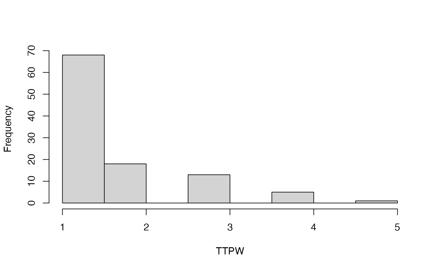
#> [[7]]
#> $breaks
#> [1] 1.0 1.5 2.0 2.5 3.0 3.5 4.0 4.5 5.0
#>
#> $counts
#> [1] 68 18 0 13 0 5 0 1
#>
#> $density
#> [1] 1.29523810 0.34285714 0.00000000 0.24761905 0.00000000 0.09523810 0.00000000
#> [8] 0.01904762
#>
#> $mids
#> [1] 1.25 1.75 2.25 2.75 3.25 3.75 4.25 4.75
#>
#> $xname
#> [1] "table(cassava_CC[, quant][, i])"
#>
#> $equidist
#> [1] TRUE
#>
#> attr(,"class")
#> [1] "histogram"
#>
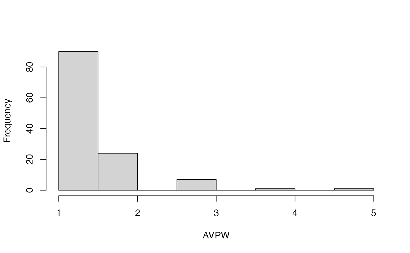
#> [[8]]
#> $breaks
#> [1] 1.0 1.5 2.0 2.5 3.0 3.5 4.0 4.5 5.0
#>
#> $counts
#> [1] 90 24 0 7 0 1 0 1
#>
#> $density
#> [1] 1.46341463 0.39024390 0.00000000 0.11382114 0.00000000 0.01626016 0.00000000
#> [8] 0.01626016
#>
#> $mids
#> [1] 1.25 1.75 2.25 2.75 3.25 3.75 4.25 4.75
#>
#> $xname
#> [1] "table(cassava_CC[, quant][, i])"
#>
#> $equidist
#> [1] TRUE
#>
#> attr(,"class")
#> [1] "histogram"
#>
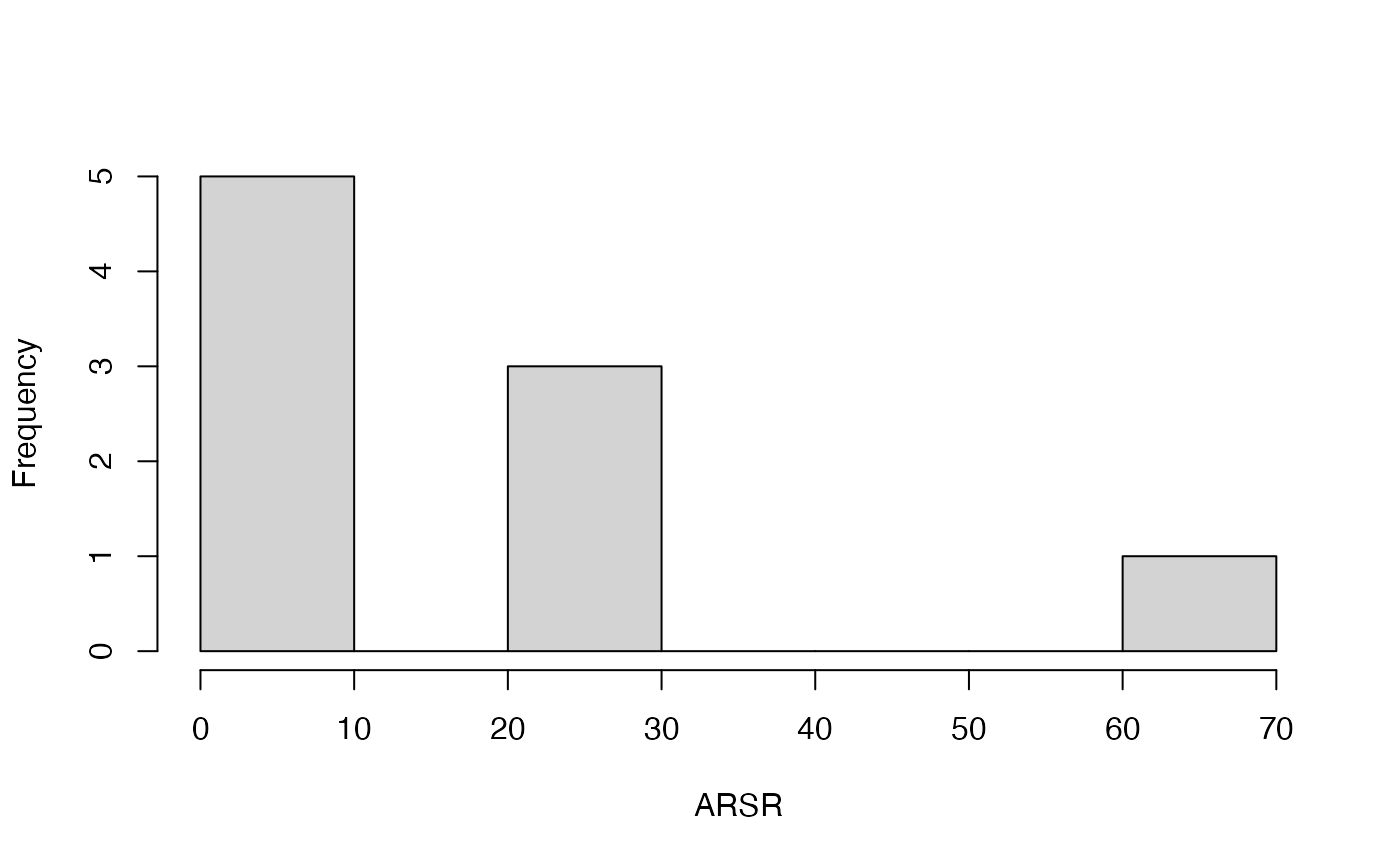
#> [[9]]
#> $breaks
#> [1] 0 10 20 30 40 50 60 70
#>
#> $counts
#> [1] 5 0 3 0 0 0 1
#>
#> $density
#> [1] 0.05555556 0.00000000 0.03333333 0.00000000 0.00000000 0.00000000 0.01111111
#>
#> $mids
#> [1] 5 15 25 35 45 55 65
#>
#> $xname
#> [1] "table(cassava_CC[, quant][, i])"
#>
#> $equidist
#> [1] TRUE
#>
#> attr(,"class")
#> [1] "histogram"
#>
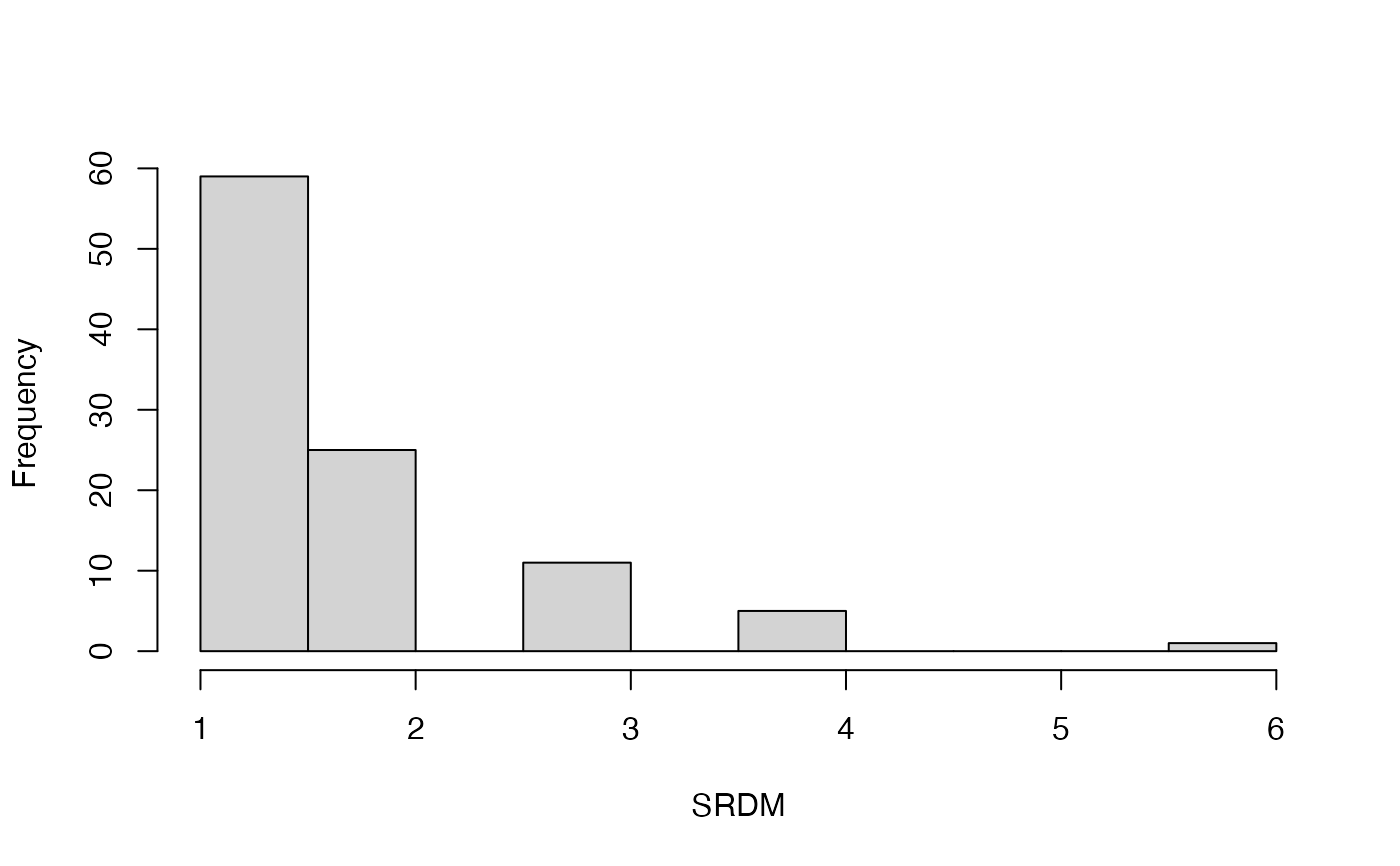
#> [[10]]
#> $breaks
#> [1] 1.0 1.5 2.0 2.5 3.0 3.5 4.0 4.5 5.0 5.5 6.0
#>
#> $counts
#> [1] 59 25 0 11 0 5 0 0 0 1
#>
#> $density
#> [1] 1.16831683 0.49504950 0.00000000 0.21782178 0.00000000 0.09900990
#> [7] 0.00000000 0.00000000 0.00000000 0.01980198
#>
#> $mids
#> [1] 1.25 1.75 2.25 2.75 3.25 3.75 4.25 4.75 5.25 5.75
#>
#> $xname
#> [1] "table(cassava_CC[, quant][, i])"
#>
#> $equidist
#> [1] TRUE
#>
#> attr(,"class")
#> [1] "histogram"
#>
#> [[1]]
#> $breaks
#> [1] 0 2 4 6 8 10 12
#>
#> $counts
#> [1] 9 4 5 4 4 4
#>
#> $density
#> [1] 0.15000000 0.06666667 0.08333333 0.06666667 0.06666667 0.06666667
#>
#> $mids
#> [1] 1 3 5 7 9 11
#>
#> $xname
#> [1] "table(cassava_CC[, quant][, i])"
#>
#> $equidist
#> [1] TRUE
#>
#> attr(,"class")
#> [1] "histogram"
#>
#> [[2]]
#> $breaks
#> [1] 0 2 4 6 8 10 12 14 16 18 20
#>
#> $counts
#> [1] 32 9 4 1 2 1 0 0 0 2
#>
#> $density
#> [1] 0.313725490 0.088235294 0.039215686 0.009803922 0.019607843 0.009803922
#> [7] 0.000000000 0.000000000 0.000000000 0.019607843
#>
#> $mids
#> [1] 1 3 5 7 9 11 13 15 17 19
#>
#> $xname
#> [1] "table(cassava_CC[, quant][, i])"
#>
#> $equidist
#> [1] TRUE
#>
#> attr(,"class")
#> [1] "histogram"
#>
#> [[3]]
#> $breaks
#> [1] 1 2 3 4 5 6 7 8
#>
#> $counts
#> [1] 42 11 7 3 3 2 1
#>
#> $density
#> [1] 0.60869565 0.15942029 0.10144928 0.04347826 0.04347826 0.02898551 0.01449275
#>
#> $mids
#> [1] 1.5 2.5 3.5 4.5 5.5 6.5 7.5
#>
#> $xname
#> [1] "table(cassava_CC[, quant][, i])"
#>
#> $equidist
#> [1] TRUE
#>
#> attr(,"class")
#> [1] "histogram"
#>
#> [[4]]
#> $breaks
#> [1] 1 2 3 4 5 6 7 8 9 10 11
#>
#> $counts
#> [1] 82 6 3 0 1 1 1 0 0 1
#>
#> $density
#> [1] 0.86315789 0.06315789 0.03157895 0.00000000 0.01052632 0.01052632
#> [7] 0.01052632 0.00000000 0.00000000 0.01052632
#>
#> $mids
#> [1] 1.5 2.5 3.5 4.5 5.5 6.5 7.5 8.5 9.5 10.5
#>
#> $xname
#> [1] "table(cassava_CC[, quant][, i])"
#>
#> $equidist
#> [1] TRUE
#>
#> attr(,"class")
#> [1] "histogram"
#>
#> [[5]]
#> $breaks
#> [1] 1.0 1.5 2.0 2.5 3.0 3.5 4.0 4.5 5.0 5.5 6.0
#>
#> $counts
#> [1] 37 14 0 11 0 6 0 8 0 1
#>
#> $density
#> [1] 0.96103896 0.36363636 0.00000000 0.28571429 0.00000000 0.15584416
#> [7] 0.00000000 0.20779221 0.00000000 0.02597403
#>
#> $mids
#> [1] 1.25 1.75 2.25 2.75 3.25 3.75 4.25 4.75 5.25 5.75
#>
#> $xname
#> [1] "table(cassava_CC[, quant][, i])"
#>
#> $equidist
#> [1] TRUE
#>
#> attr(,"class")
#> [1] "histogram"
#>
#> [[6]]
#> $breaks
#> [1] 1.0 1.5 2.0 2.5 3.0 3.5 4.0 4.5 5.0 5.5 6.0
#>
#> $counts
#> [1] 64 16 0 10 0 2 0 2 0 4
#>
#> $density
#> [1] 1.30612245 0.32653061 0.00000000 0.20408163 0.00000000 0.04081633
#> [7] 0.00000000 0.04081633 0.00000000 0.08163265
#>
#> $mids
#> [1] 1.25 1.75 2.25 2.75 3.25 3.75 4.25 4.75 5.25 5.75
#>
#> $xname
#> [1] "table(cassava_CC[, quant][, i])"
#>
#> $equidist
#> [1] TRUE
#>
#> attr(,"class")
#> [1] "histogram"
#>
#> [[7]]
#> $breaks
#> [1] 1.0 1.5 2.0 2.5 3.0 3.5 4.0 4.5 5.0
#>
#> $counts
#> [1] 68 18 0 13 0 5 0 1
#>
#> $density
#> [1] 1.29523810 0.34285714 0.00000000 0.24761905 0.00000000 0.09523810 0.00000000
#> [8] 0.01904762
#>
#> $mids
#> [1] 1.25 1.75 2.25 2.75 3.25 3.75 4.25 4.75
#>
#> $xname
#> [1] "table(cassava_CC[, quant][, i])"
#>
#> $equidist
#> [1] TRUE
#>
#> attr(,"class")
#> [1] "histogram"
#>
#> [[8]]
#> $breaks
#> [1] 1.0 1.5 2.0 2.5 3.0 3.5 4.0 4.5 5.0
#>
#> $counts
#> [1] 90 24 0 7 0 1 0 1
#>
#> $density
#> [1] 1.46341463 0.39024390 0.00000000 0.11382114 0.00000000 0.01626016 0.00000000
#> [8] 0.01626016
#>
#> $mids
#> [1] 1.25 1.75 2.25 2.75 3.25 3.75 4.25 4.75
#>
#> $xname
#> [1] "table(cassava_CC[, quant][, i])"
#>
#> $equidist
#> [1] TRUE
#>
#> attr(,"class")
#> [1] "histogram"
#>
#> [[9]]
#> $breaks
#> [1] 0 10 20 30 40 50 60 70
#>
#> $counts
#> [1] 5 0 3 0 0 0 1
#>
#> $density
#> [1] 0.05555556 0.00000000 0.03333333 0.00000000 0.00000000 0.00000000 0.01111111
#>
#> $mids
#> [1] 5 15 25 35 45 55 65
#>
#> $xname
#> [1] "table(cassava_CC[, quant][, i])"
#>
#> $equidist
#> [1] TRUE
#>
#> attr(,"class")
#> [1] "histogram"
#>
#> [[10]]
#> $breaks
#> [1] 1.0 1.5 2.0 2.5 3.0 3.5 4.0 4.5 5.0 5.5 6.0
#>
#> $counts
#> [1] 59 25 0 11 0 5 0 0 0 1
#>
#> $density
#> [1] 1.16831683 0.49504950 0.00000000 0.21782178 0.00000000 0.09900990
#> [7] 0.00000000 0.00000000 0.00000000 0.01980198
#>
#> $mids
#> [1] 1.25 1.75 2.25 2.75 3.25 3.75 4.25 4.75 5.25 5.75
#>
#> $xname
#> [1] "table(cassava_CC[, quant][, i])"
#>
#> $equidist
#> [1] TRUE
#>
#> attr(,"class")
#> [1] "histogram"
#>