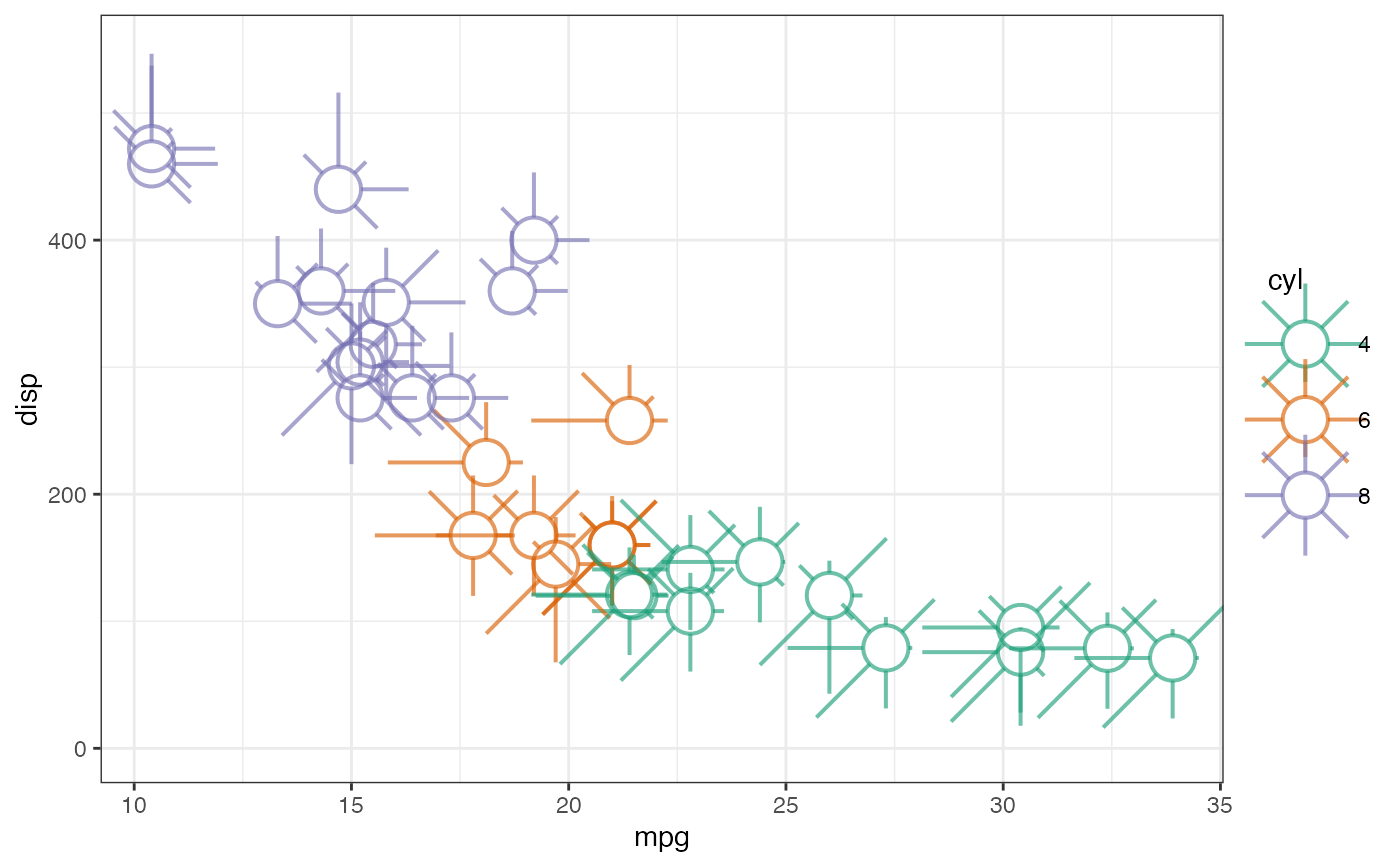
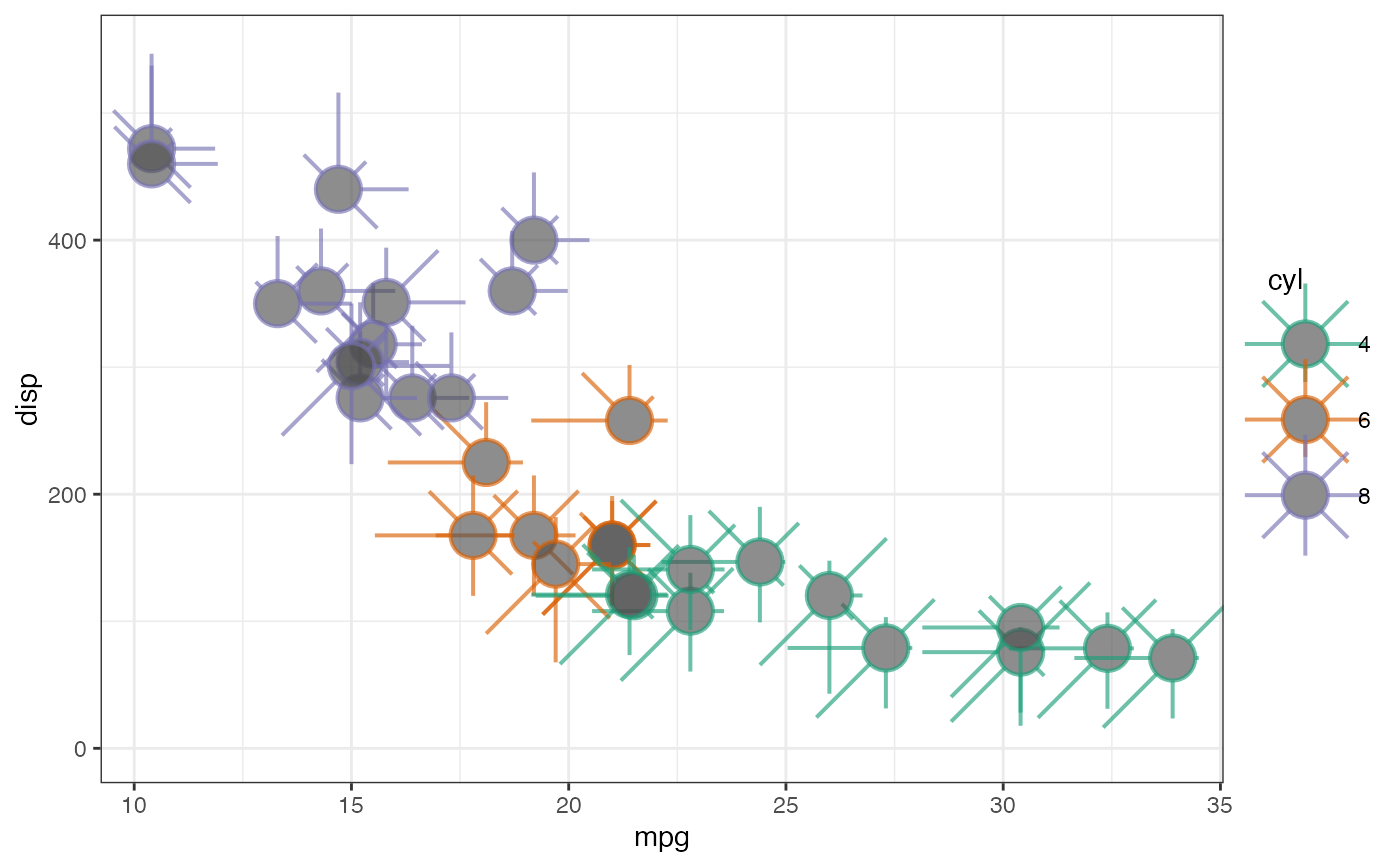
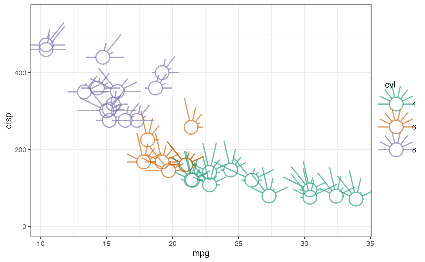
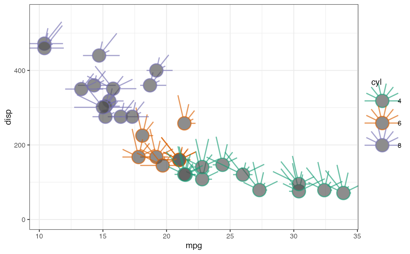
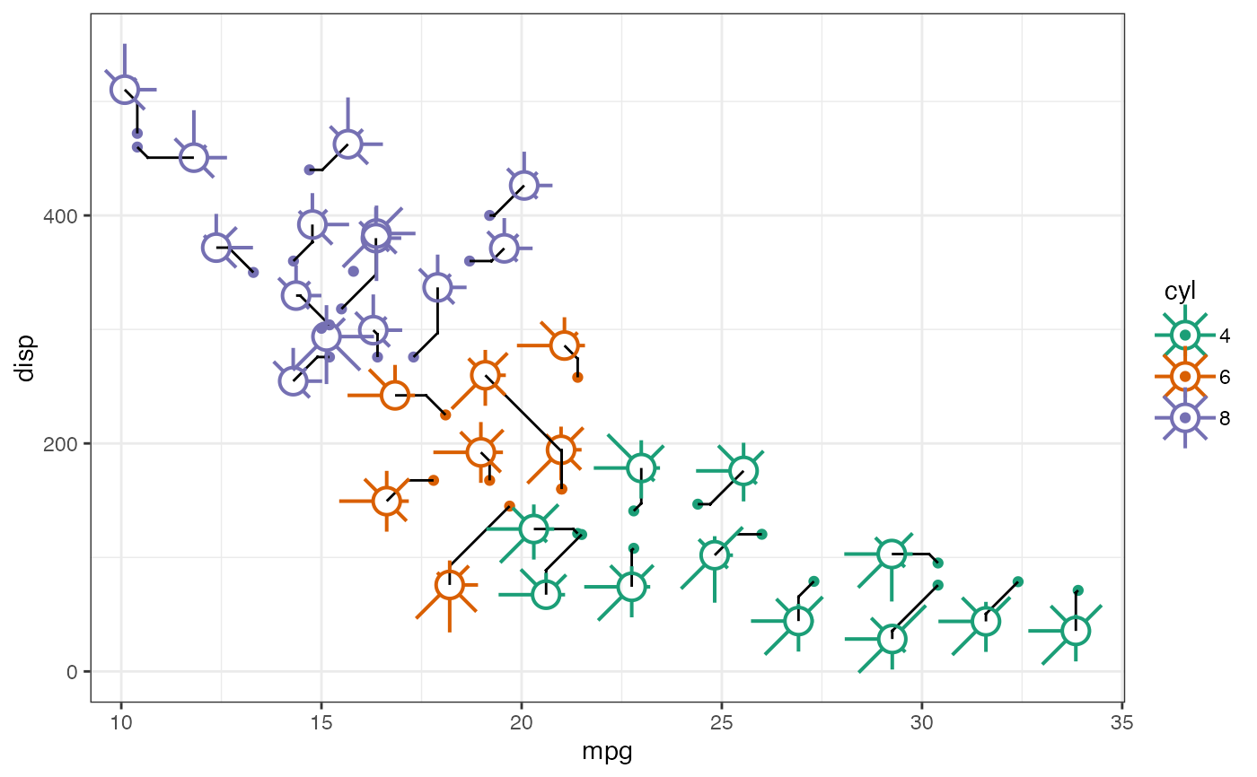
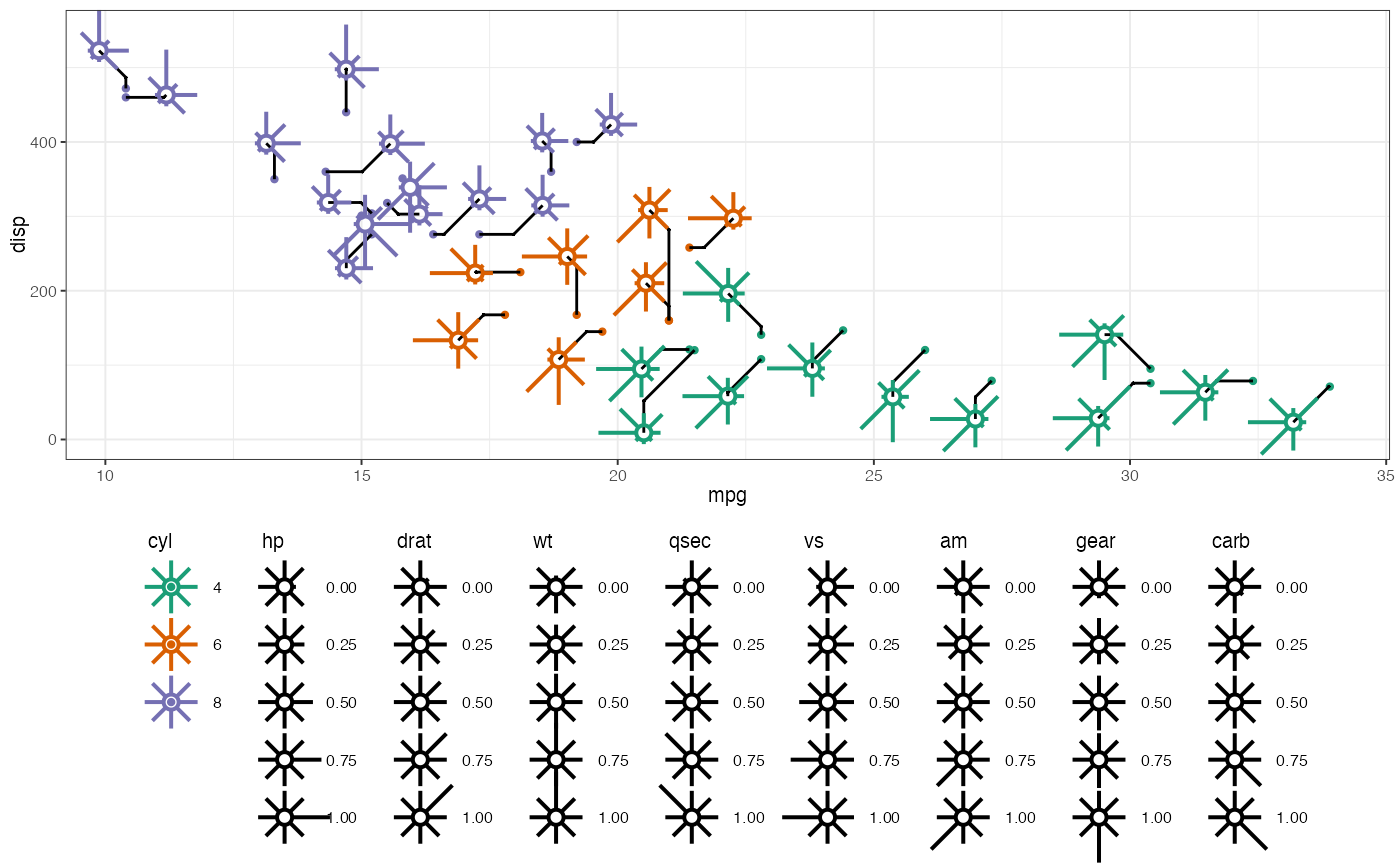
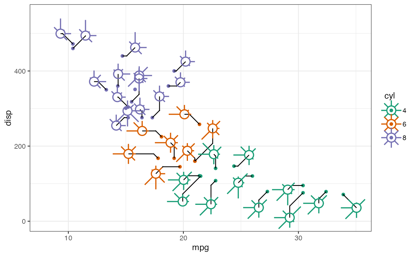
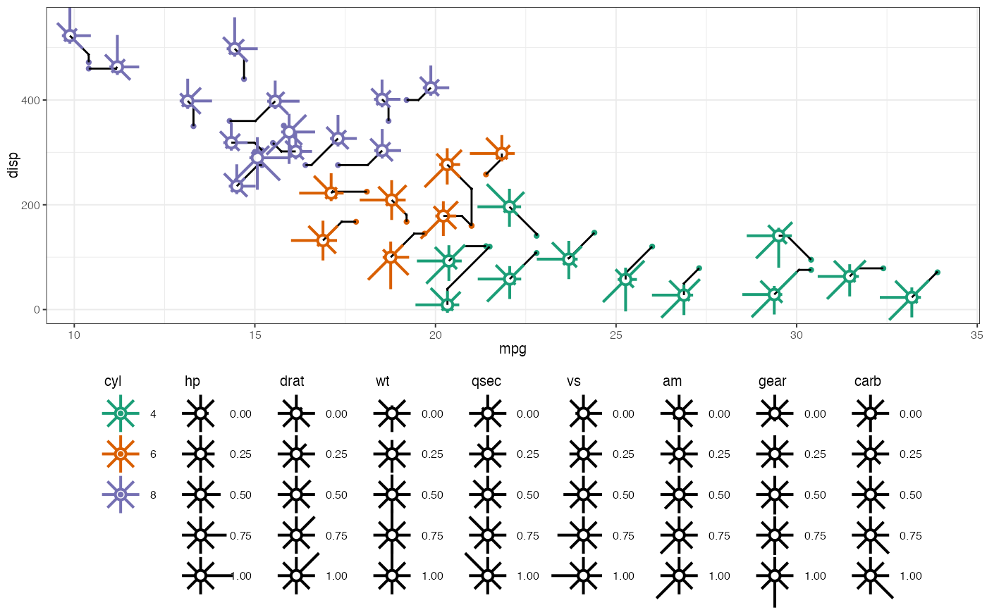
The metroglyph geom is used to plot multivariate data as metroglyphs (Anderson 1957; duToit et al. 1986) in a scatterplot.
Usage
geom_metroglyph(
  mapping = NULL,
  data = NULL,
  stat = "identity",
  position = "identity",
  ...,
  cols = character(0L),
  circle.size = 1,
  colour.circle = NULL,
  colour.ray = NULL,
  colour.points = NULL,
  linewidth.circle = 1,
  linewidth.ray = 1,
  lineend = "butt",
  full = TRUE,
  draw.grid = FALSE,
  grid.point.size = 1,
  show.legend = NA,
  legend.glyph.dims = setNames(rep(0.5, length(cols)), cols),
  repel = FALSE,
  repel.control = ggmultiglyph.repel.control(),
  inherit.aes = TRUE
)
Arguments
- mapping
Set of aesthetic mappings created by
aes(). If specified andinherit.aes = TRUE(the default), it is combined with the default mapping at the top level of the plot. You must supplymappingif there is no plot mapping.- data
The data to be displayed in this layer. There are three options:
If
NULL, the default, the data is inherited from the plot data as specified in the call toggplot().A
data.frame, or other object, will override the plot data. All objects will be fortified to produce a data frame. Seefortify()for which variables will be created.A
functionwill be called with a single argument, the plot data. The return value must be adata.frame, and will be used as the layer data. Afunctioncan be created from aformula(e.g.~ head(.x, 10)).- stat
The statistical transformation to use on the data for this layer. When using a
geom_*()function to construct a layer, thestatargument can be used to override the default coupling between geoms and stats. Thestatargument accepts the following:A
Statggproto subclass, for exampleStatCount.A string naming the stat. To give the stat as a string, strip the function name of the
stat_prefix. For example, to usestat_count(), give the stat as"count".For more information and other ways to specify the stat, see the layer stat documentation.
- position
A position adjustment to use on the data for this layer. This can be used in various ways, including to prevent overplotting and improving the display. The
positionargument accepts the following:The result of calling a position function, such as
position_jitter(). This method allows for passing extra arguments to the position.A string naming the position adjustment. To give the position as a string, strip the function name of the
position_prefix. For example, to useposition_jitter(), give the position as"jitter".For more information and other ways to specify the position, see the layer position documentation.
- ...
Other arguments passed on to
layer(). These are often aesthetics, used to set an aesthetic to a fixed value, likecolour = "green"orsize = 3. They may also be parameters to the paired geom/stat.- cols
A character vector containing the names of at least two columns specifying the variables to be plotted in the glyphs. The selected columns must be either numeric or factor variables.
- circle.size
The size of the central circle (radius).
- colour.circle
The colour of circles.
- colour.ray
The colour of rays.
- colour.points
The colour of grid points.
- linewidth.circle
The circle line width.
- linewidth.ray
The ray line width.
- lineend
The line end style for the rays. Either
"round","butt"or"square".- full
logical. If
TRUE, full star glyphs (360°) are plotted, otherwise half star glyphs (180°) are plotted.- draw.grid
logical. If
TRUE, grid points are plotted along the rays if all the variables specified incolsare an ordered factor. Default isFALSE.- grid.point.size
The size of the grid points in native units.
- show.legend
logical. Should this layer be included in the legends?
NA, the default, includes if any aesthetics are mapped.FALSEnever includes, andTRUEalways includes. It can also be a named logical vector to finely select the aesthetics to display. To include legend keys for all levels, even when no data exists, useTRUE. IfNA, all levels are shown in legend, but unobserved levels are omitted.- legend.glyph.dims
The dimensions of the legend glyph plot. Can be a numeric vector of unit length (where all the dimensions will have same value) or a numeric vector of same length as "cols" with the "cols" as names.
- repel
logical. If
TRUE, the glyphs are repel away from each other to avoid overlaps. Default isFALSE.- repel.control
A list of control settings for the repel algorithm. Ignored if
repel = FALSE. Seeggmultiglyph.repel.controlfor details on the various control parameters.- inherit.aes
If
FALSE, overrides the default aesthetics, rather than combining with them. This is most useful for helper functions that define both data and aesthetics and shouldn't inherit behaviour from the default plot specification, e.g.annotation_borders().
Aesthetics
geom_metroglyph() understands the following
aesthetics (required aesthetics are in bold):
x
y
alpha
colour
fill
group
circle.size
See vignette("ggplot2-specs", package = "ggplot2") for further
details on setting these aesthetics.
The following additional aesthetics are considered if repel = TRUE:
point.size
segment.linetype
segment.colour
segment.size
segment.alpha
segment.curvature
segment.angle
segment.ncp
segment.shape
segment.square
segment.squareShape
segment.inflect
segment.debug
See ggrepel
examples page
for further details on setting these aesthetics.
References
Anderson E (1957).
“A semigraphical method for the analysis of complex problems.”
Proceedings of the National Academy of Sciences of the United States of America, 43(10), 923.
duToit SHC, Steyn AGW, Stumpf RH (1986).
Graphical Exploratory Data Analysis, Springer Texts in Statistics.
Springer-Verlag, New York.
ISBN 978-1-4612-9371-2.
Examples
library(ggplot2)
#~~~~~~~~~~~~~~~~~~~~~~~~~~~~~~~~~~~~~~~~~~~~~~~~~~~~~~~~~~~~~~~~~~~~~~~~~~~~
# Prepare the data ----
#~~~~~~~~~~~~~~~~~~~~~~~~~~~~~~~~~~~~~~~~~~~~~~~~~~~~~~~~~~~~~~~~~~~~~~~~~~~~
# Variables to map to glyphs
zs <- c("hp", "drat", "wt", "qsec", "vs", "am", "gear", "carb")
# Keep a copy of the original data
mtcars_fct <- mtcars
# Scaled numeric data
mtcars[zs] <- lapply(mtcars[zs], scales::rescale)
mtcars$cyl <- factor(mtcars$cyl)
mtcars$lab <- row.names(mtcars)
# Ordered factor data
mtcars_fct[zs[1:3]] <-
lapply(mtcars_fct[zs[1:3]], function(x)
ordered(cut(x, breaks = 3,
labels = c("low", "medium", "high"))))
mtcars_fct[zs[4:8]] <-
lapply(mtcars_fct[zs[4:8]], function(x)
ordered(cut(x, breaks = 4,
labels = c("tiny", "small", "medium", "large"))))
mtcars_fct$cyl <- factor(mtcars_fct$cyl)
mtcars_fct$lab <- row.names(mtcars_fct)
#~~~~~~~~~~~~~~~~~~~~~~~~~~~~~~~~~~~~~~~~~~~~~~~~~~~~~~~~~~~~~~~~~~~~~~~~~~~~
# Mapped colour ----
#~~~~~~~~~~~~~~~~~~~~~~~~~~~~~~~~~~~~~~~~~~~~~~~~~~~~~~~~~~~~~~~~~~~~~~~~~~~~
ggplot(data = mtcars) +
geom_metroglyph(aes(x = mpg, y = disp, colour = cyl),
cols = zs, circle.size = 3, colour.ray = NULL,
linewidth.circle = 2, linewidth.ray = 2,
size = 10, alpha = 0.8) +
ylim(c(-0, 550))
 ggplot(data = mtcars) +
geom_metroglyph(aes(x = mpg, y = disp, colour = cyl),
cols = zs, circle.size = 3, colour.ray = NULL,
linewidth.circle = 2, linewidth.ray = 2, fill = "gray30",
size = 10, alpha = 0.8) +
ylim(c(-0, 550))
ggplot(data = mtcars) +
geom_metroglyph(aes(x = mpg, y = disp, colour = cyl),
cols = zs, circle.size = 3, colour.ray = NULL,
linewidth.circle = 2, linewidth.ray = 2, fill = "gray30",
size = 10, alpha = 0.8) +
ylim(c(-0, 550))
 ggplot(data = mtcars) +
geom_metroglyph(aes(x = mpg, y = disp, colour = cyl),
cols = zs, circle.size = 3, colour.ray = NULL,
linewidth.circle = 2, linewidth.ray = 2,
full = FALSE,
size = 10, alpha = 0.8) +
ylim(c(-0, 550))
ggplot(data = mtcars) +
geom_metroglyph(aes(x = mpg, y = disp, colour = cyl),
cols = zs, circle.size = 3, colour.ray = NULL,
linewidth.circle = 2, linewidth.ray = 2,
full = FALSE,
size = 10, alpha = 0.8) +
ylim(c(-0, 550))
 ggplot(data = mtcars) +
geom_metroglyph(aes(x = mpg, y = disp, colour = cyl),
cols = zs, circle.size = 3, colour.ray = NULL,
full = FALSE,
linewidth.circle = 2, linewidth.ray = 2, fill = "gray30",
size = 10, alpha = 0.8) +
ylim(c(-0, 550))
ggplot(data = mtcars) +
geom_metroglyph(aes(x = mpg, y = disp, colour = cyl),
cols = zs, circle.size = 3, colour.ray = NULL,
full = FALSE,
linewidth.circle = 2, linewidth.ray = 2, fill = "gray30",
size = 10, alpha = 0.8) +
ylim(c(-0, 550))
 # \donttest{
#~~~~~~~~~~~~~~~~~~~~~~~~~~~~~~~~~~~~~~~~~~~~~~~~~~~~~~~~~~~~~~~~~~~~~~~~~~~~
# Mapped colour + fill ----
#~~~~~~~~~~~~~~~~~~~~~~~~~~~~~~~~~~~~~~~~~~~~~~~~~~~~~~~~~~~~~~~~~~~~~~~~~~~~
ggplot(data = mtcars) +
geom_metroglyph(aes(x = mpg, y = disp, colour = cyl, fill = cyl),
cols = zs, circle.size = 3, colour.ray = NULL,
linewidth.circle = 2, linewidth.ray = 2,
size = 10, alpha = 0.8) +
ylim(c(-0, 550))
# \donttest{
#~~~~~~~~~~~~~~~~~~~~~~~~~~~~~~~~~~~~~~~~~~~~~~~~~~~~~~~~~~~~~~~~~~~~~~~~~~~~
# Mapped colour + fill ----
#~~~~~~~~~~~~~~~~~~~~~~~~~~~~~~~~~~~~~~~~~~~~~~~~~~~~~~~~~~~~~~~~~~~~~~~~~~~~
ggplot(data = mtcars) +
geom_metroglyph(aes(x = mpg, y = disp, colour = cyl, fill = cyl),
cols = zs, circle.size = 3, colour.ray = NULL,
linewidth.circle = 2, linewidth.ray = 2,
size = 10, alpha = 0.8) +
ylim(c(-0, 550))
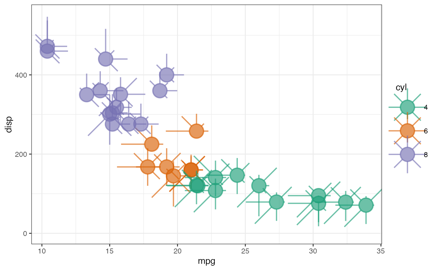 ggplot(data = mtcars) +
geom_metroglyph(aes(x = mpg, y = disp, colour = cyl, fill = cyl),
cols = zs, circle.size = 3, colour.ray = NULL,
full = FALSE,
linewidth.circle = 2, linewidth.ray = 2,
size = 10, alpha = 0.8) +
ylim(c(-0, 550))
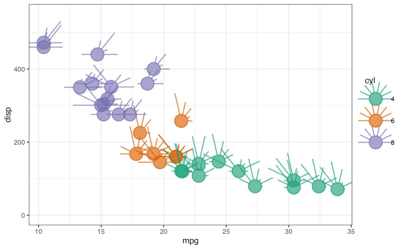
ggplot(data = mtcars) +
geom_metroglyph(aes(x = mpg, y = disp, colour = cyl, fill = cyl),
cols = zs, circle.size = 3, colour.ray = NULL,
full = FALSE,
linewidth.circle = 2, linewidth.ray = 2,
size = 10, alpha = 0.8) +
ylim(c(-0, 550))
 #~~~~~~~~~~~~~~~~~~~~~~~~~~~~~~~~~~~~~~~~~~~~~~~~~~~~~~~~~~~~~~~~~~~~~~~~~~~~
# Mapped fill ----
#~~~~~~~~~~~~~~~~~~~~~~~~~~~~~~~~~~~~~~~~~~~~~~~~~~~~~~~~~~~~~~~~~~~~~~~~~~~~
ggplot(data = mtcars) +
geom_metroglyph(aes(x = mpg, y = disp, fill = cyl),
cols = zs, circle.size = 3, colour.ray = NULL,
linewidth.circle = 2, linewidth.ray = 2,
size = 10, alpha = 0.8) +
ylim(c(-0, 550))
#~~~~~~~~~~~~~~~~~~~~~~~~~~~~~~~~~~~~~~~~~~~~~~~~~~~~~~~~~~~~~~~~~~~~~~~~~~~~
# Mapped fill ----
#~~~~~~~~~~~~~~~~~~~~~~~~~~~~~~~~~~~~~~~~~~~~~~~~~~~~~~~~~~~~~~~~~~~~~~~~~~~~
ggplot(data = mtcars) +
geom_metroglyph(aes(x = mpg, y = disp, fill = cyl),
cols = zs, circle.size = 3, colour.ray = NULL,
linewidth.circle = 2, linewidth.ray = 2,
size = 10, alpha = 0.8) +
ylim(c(-0, 550))
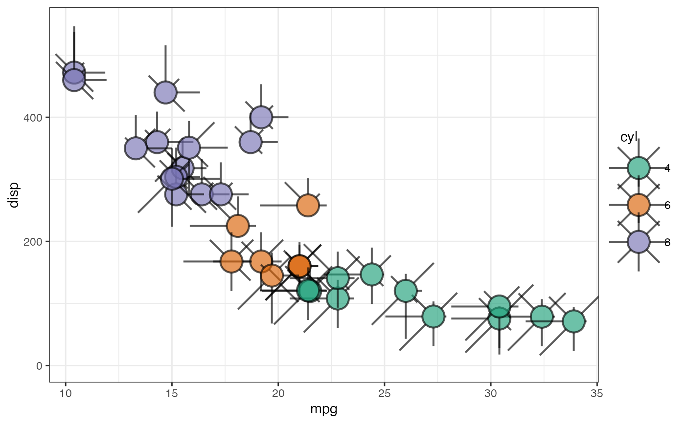 ggplot(data = mtcars) +
geom_metroglyph(aes(x = mpg, y = disp, fill = cyl),
cols = zs, circle.size = 3, colour.ray = NULL,
linewidth.circle = 2, linewidth.ray = 2,
colour.circle = "transparent",
size = 10, alpha = 0.8) +
ylim(c(-0, 550))
ggplot(data = mtcars) +
geom_metroglyph(aes(x = mpg, y = disp, fill = cyl),
cols = zs, circle.size = 3, colour.ray = NULL,
linewidth.circle = 2, linewidth.ray = 2,
colour.circle = "transparent",
size = 10, alpha = 0.8) +
ylim(c(-0, 550))
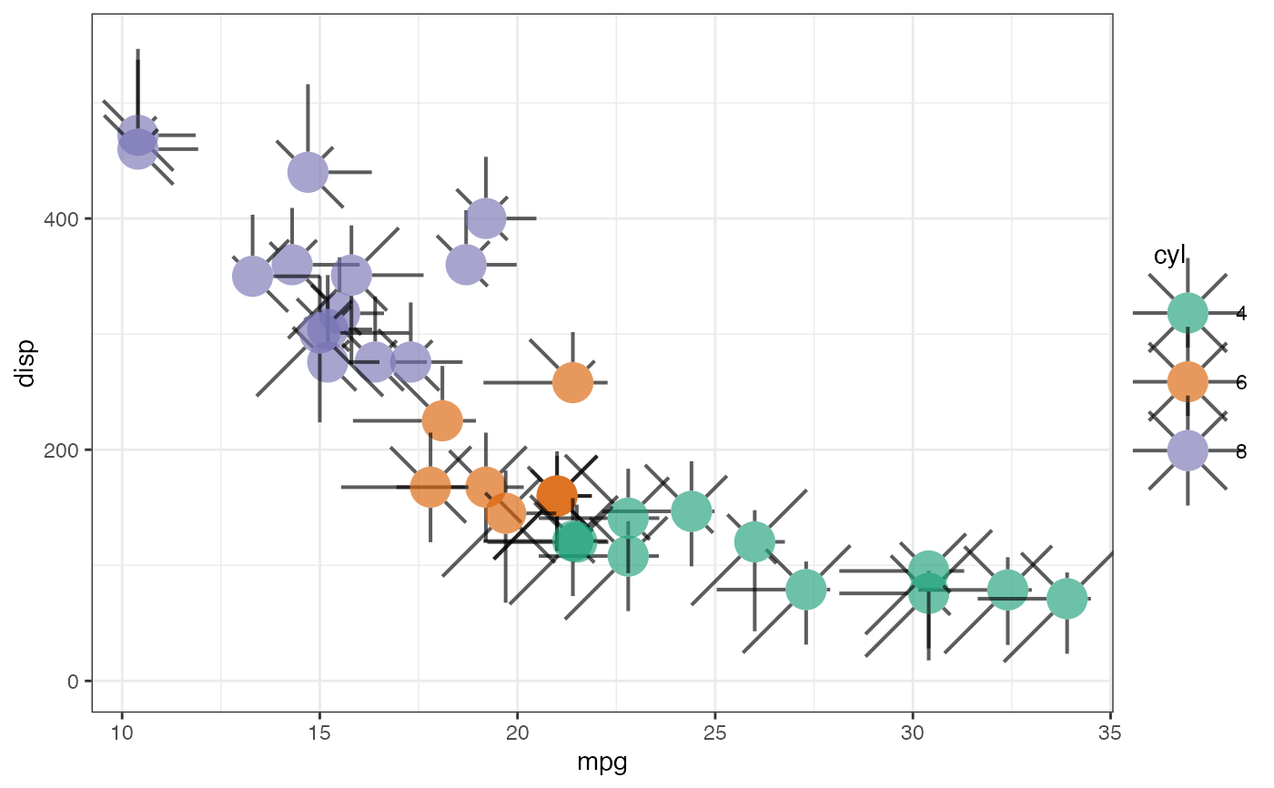 ggplot(data = mtcars) +
geom_metroglyph(aes(x = mpg, y = disp, fill = cyl),
cols = zs, circle.size = 3, colour.ray = NULL,
full = FALSE,
linewidth.circle = 2, linewidth.ray = 2,
size = 10, alpha = 0.8) +
ylim(c(-0, 550))
ggplot(data = mtcars) +
geom_metroglyph(aes(x = mpg, y = disp, fill = cyl),
cols = zs, circle.size = 3, colour.ray = NULL,
full = FALSE,
linewidth.circle = 2, linewidth.ray = 2,
size = 10, alpha = 0.8) +
ylim(c(-0, 550))
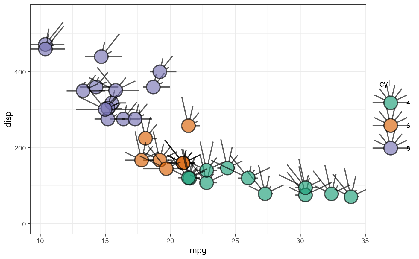 ggplot(data = mtcars) +
geom_metroglyph(aes(x = mpg, y = disp, fill = cyl),
cols = zs, circle.size = 3, colour.ray = NULL,
full = FALSE, colour.circle = "transparent",
linewidth.circle = 2, linewidth.ray = 2,
size = 10, alpha = 0.8) +
ylim(c(-0, 550))
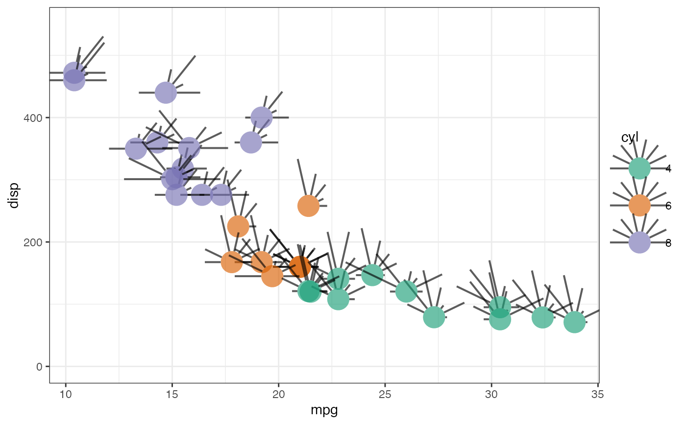
ggplot(data = mtcars) +
geom_metroglyph(aes(x = mpg, y = disp, fill = cyl),
cols = zs, circle.size = 3, colour.ray = NULL,
full = FALSE, colour.circle = "transparent",
linewidth.circle = 2, linewidth.ray = 2,
size = 10, alpha = 0.8) +
ylim(c(-0, 550))
 #~~~~~~~~~~~~~~~~~~~~~~~~~~~~~~~~~~~~~~~~~~~~~~~~~~~~~~~~~~~~~~~~~~~~~~~~~~~~
# Rays with multivariate colours ----
#~~~~~~~~~~~~~~~~~~~~~~~~~~~~~~~~~~~~~~~~~~~~~~~~~~~~~~~~~~~~~~~~~~~~~~~~~~~~
ggplot(data = mtcars) +
geom_metroglyph(aes(x = mpg, y = disp),
cols = zs, circle.size = 3,
linewidth.circle = 0, linewidth.ray = 2,
colour.circle = "transparent", fill = "gray",
colour.ray = RColorBrewer::brewer.pal(8, "Dark2"),
size = 10, alpha = 0.8) +
ylim(c(-0, 550))
#~~~~~~~~~~~~~~~~~~~~~~~~~~~~~~~~~~~~~~~~~~~~~~~~~~~~~~~~~~~~~~~~~~~~~~~~~~~~
# Rays with multivariate colours ----
#~~~~~~~~~~~~~~~~~~~~~~~~~~~~~~~~~~~~~~~~~~~~~~~~~~~~~~~~~~~~~~~~~~~~~~~~~~~~
ggplot(data = mtcars) +
geom_metroglyph(aes(x = mpg, y = disp),
cols = zs, circle.size = 3,
linewidth.circle = 0, linewidth.ray = 2,
colour.circle = "transparent", fill = "gray",
colour.ray = RColorBrewer::brewer.pal(8, "Dark2"),
size = 10, alpha = 0.8) +
ylim(c(-0, 550))
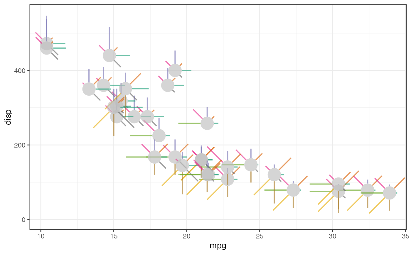 ggplot(data = mtcars) +
geom_metroglyph(aes(x = mpg, y = disp),
cols = zs, circle.size = 3,
linewidth.circle = 0, linewidth.ray = 2,
colour.circle = "transparent", fill = "gray",
colour.ray = RColorBrewer::brewer.pal(8, "Dark2"),
size = 10, alpha = 0.8, full = FALSE) +
ylim(c(-0, 550))
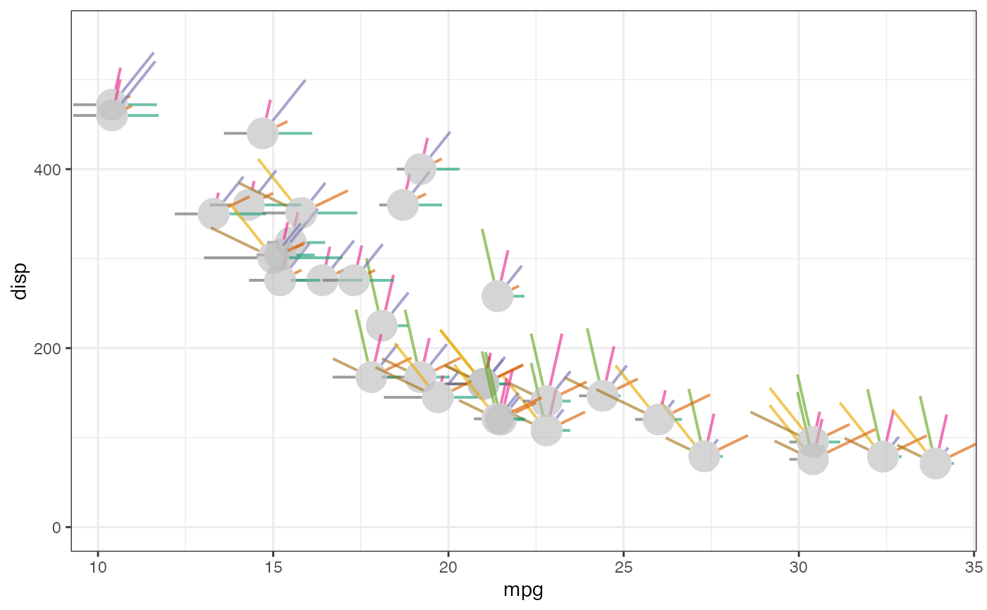
ggplot(data = mtcars) +
geom_metroglyph(aes(x = mpg, y = disp),
cols = zs, circle.size = 3,
linewidth.circle = 0, linewidth.ray = 2,
colour.circle = "transparent", fill = "gray",
colour.ray = RColorBrewer::brewer.pal(8, "Dark2"),
size = 10, alpha = 0.8, full = FALSE) +
ylim(c(-0, 550))
 #~~~~~~~~~~~~~~~~~~~~~~~~~~~~~~~~~~~~~~~~~~~~~~~~~~~~~~~~~~~~~~~~~~~~~~~~~~~~
# Faceted ----
#~~~~~~~~~~~~~~~~~~~~~~~~~~~~~~~~~~~~~~~~~~~~~~~~~~~~~~~~~~~~~~~~~~~~~~~~~~~~
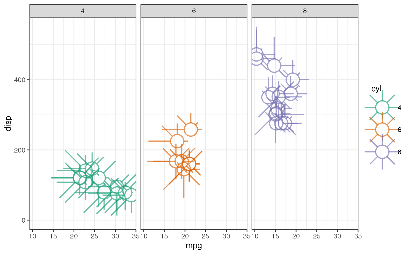
ggplot(data = mtcars) +
geom_metroglyph(aes(x = mpg, y = disp, colour = cyl),
cols = zs, circle.size = 3, colour.ray = NULL,
linewidth.circle = 2, linewidth.ray = 2,
size = 10, alpha = 0.8) +
ylim(c(-0, 550)) +
facet_grid(. ~ cyl)
#~~~~~~~~~~~~~~~~~~~~~~~~~~~~~~~~~~~~~~~~~~~~~~~~~~~~~~~~~~~~~~~~~~~~~~~~~~~~
# Faceted ----
#~~~~~~~~~~~~~~~~~~~~~~~~~~~~~~~~~~~~~~~~~~~~~~~~~~~~~~~~~~~~~~~~~~~~~~~~~~~~
ggplot(data = mtcars) +
geom_metroglyph(aes(x = mpg, y = disp, colour = cyl),
cols = zs, circle.size = 3, colour.ray = NULL,
linewidth.circle = 2, linewidth.ray = 2,
size = 10, alpha = 0.8) +
ylim(c(-0, 550)) +
facet_grid(. ~ cyl)
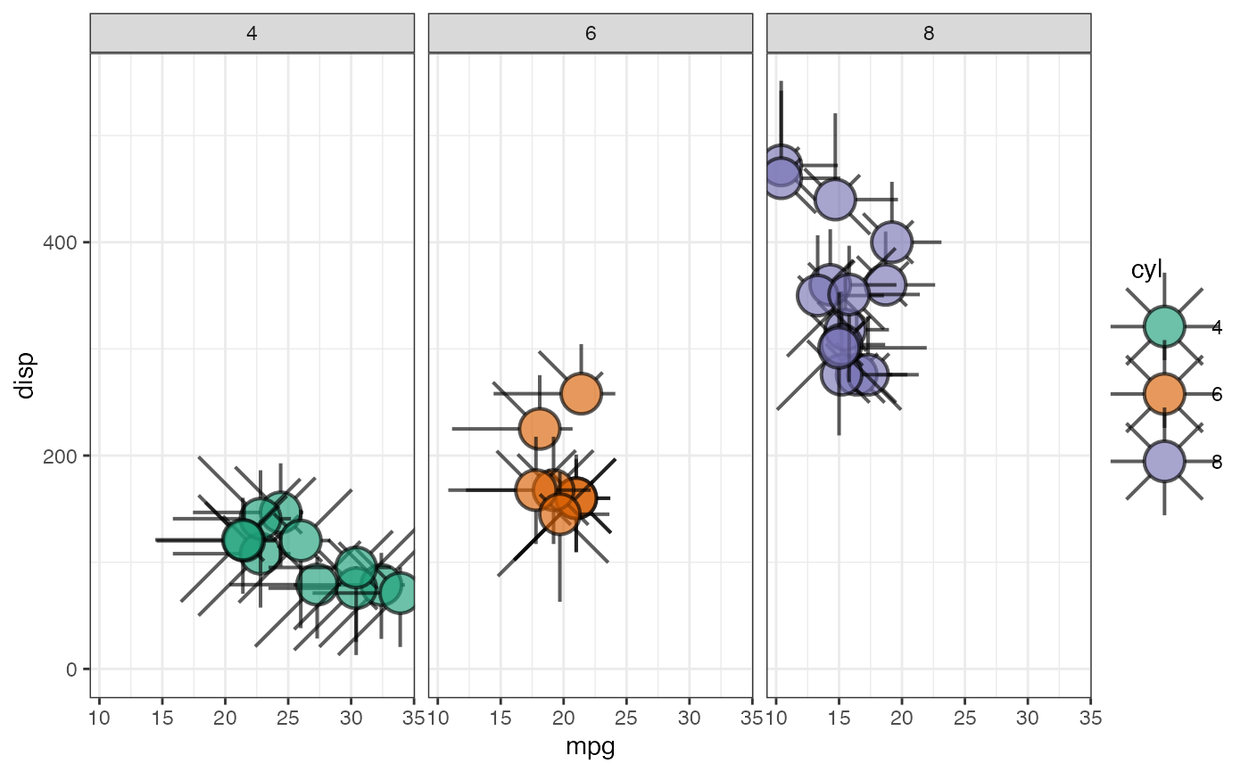
 ggplot(data = mtcars) +
geom_metroglyph(aes(x = mpg, y = disp, fill = cyl),
cols = zs, circle.size = 3, colour.ray = NULL,
linewidth.circle = 2, linewidth.ray = 2,
size = 10, alpha = 0.8) +
ylim(c(-0, 550)) +
facet_grid(. ~ cyl)
ggplot(data = mtcars) +
geom_metroglyph(aes(x = mpg, y = disp, fill = cyl),
cols = zs, circle.size = 3, colour.ray = NULL,
linewidth.circle = 2, linewidth.ray = 2,
size = 10, alpha = 0.8) +
ylim(c(-0, 550)) +
facet_grid(. ~ cyl)
 #~~~~~~~~~~~~~~~~~~~~~~~~~~~~~~~~~~~~~~~~~~~~~~~~~~~~~~~~~~~~~~~~~~~~~~~~~~~~
# Repel glyphs ----
#~~~~~~~~~~~~~~~~~~~~~~~~~~~~~~~~~~~~~~~~~~~~~~~~~~~~~~~~~~~~~~~~~~~~~~~~~~~~
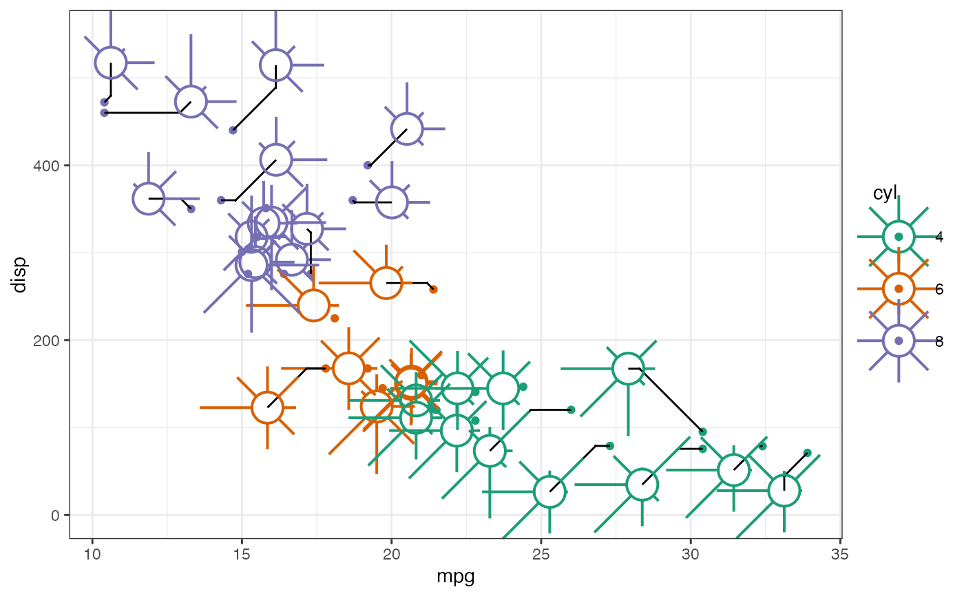
ggplot(data = mtcars) +
geom_point(aes(x = mpg, y = disp, colour = cyl)) +
geom_metroglyph(aes(x = mpg, y = disp, colour = cyl),
cols = zs, circle.size = 3, colour.ray = NULL,
linewidth.circle = 2, linewidth.ray = 2,
size = 10, alpha = 1, repel = TRUE) +
ylim(c(-0, 550))
#> Warning: 14 glyphs have too many overlaps.
#> Consider increasing "max.overlaps"
#~~~~~~~~~~~~~~~~~~~~~~~~~~~~~~~~~~~~~~~~~~~~~~~~~~~~~~~~~~~~~~~~~~~~~~~~~~~~
# Repel glyphs ----
#~~~~~~~~~~~~~~~~~~~~~~~~~~~~~~~~~~~~~~~~~~~~~~~~~~~~~~~~~~~~~~~~~~~~~~~~~~~~
ggplot(data = mtcars) +
geom_point(aes(x = mpg, y = disp, colour = cyl)) +
geom_metroglyph(aes(x = mpg, y = disp, colour = cyl),
cols = zs, circle.size = 3, colour.ray = NULL,
linewidth.circle = 2, linewidth.ray = 2,
size = 10, alpha = 1, repel = TRUE) +
ylim(c(-0, 550))
#> Warning: 14 glyphs have too many overlaps.
#> Consider increasing "max.overlaps"
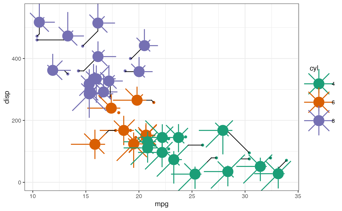
 ggplot(data = mtcars) +
geom_point(aes(x = mpg, y = disp, colour = cyl)) +
geom_metroglyph(aes(x = mpg, y = disp, colour = cyl, fill = cyl),
cols = zs, circle.size = 3, colour.ray = NULL,
linewidth.circle = 2, linewidth.ray = 2,
colour.circle = "transparent",
size = 10, alpha = 1, repel = TRUE) +
ylim(c(-0, 550))
#> Warning: 14 glyphs have too many overlaps.
#> Consider increasing "max.overlaps"
ggplot(data = mtcars) +
geom_point(aes(x = mpg, y = disp, colour = cyl)) +
geom_metroglyph(aes(x = mpg, y = disp, colour = cyl, fill = cyl),
cols = zs, circle.size = 3, colour.ray = NULL,
linewidth.circle = 2, linewidth.ray = 2,
colour.circle = "transparent",
size = 10, alpha = 1, repel = TRUE) +
ylim(c(-0, 550))
#> Warning: 14 glyphs have too many overlaps.
#> Consider increasing "max.overlaps"
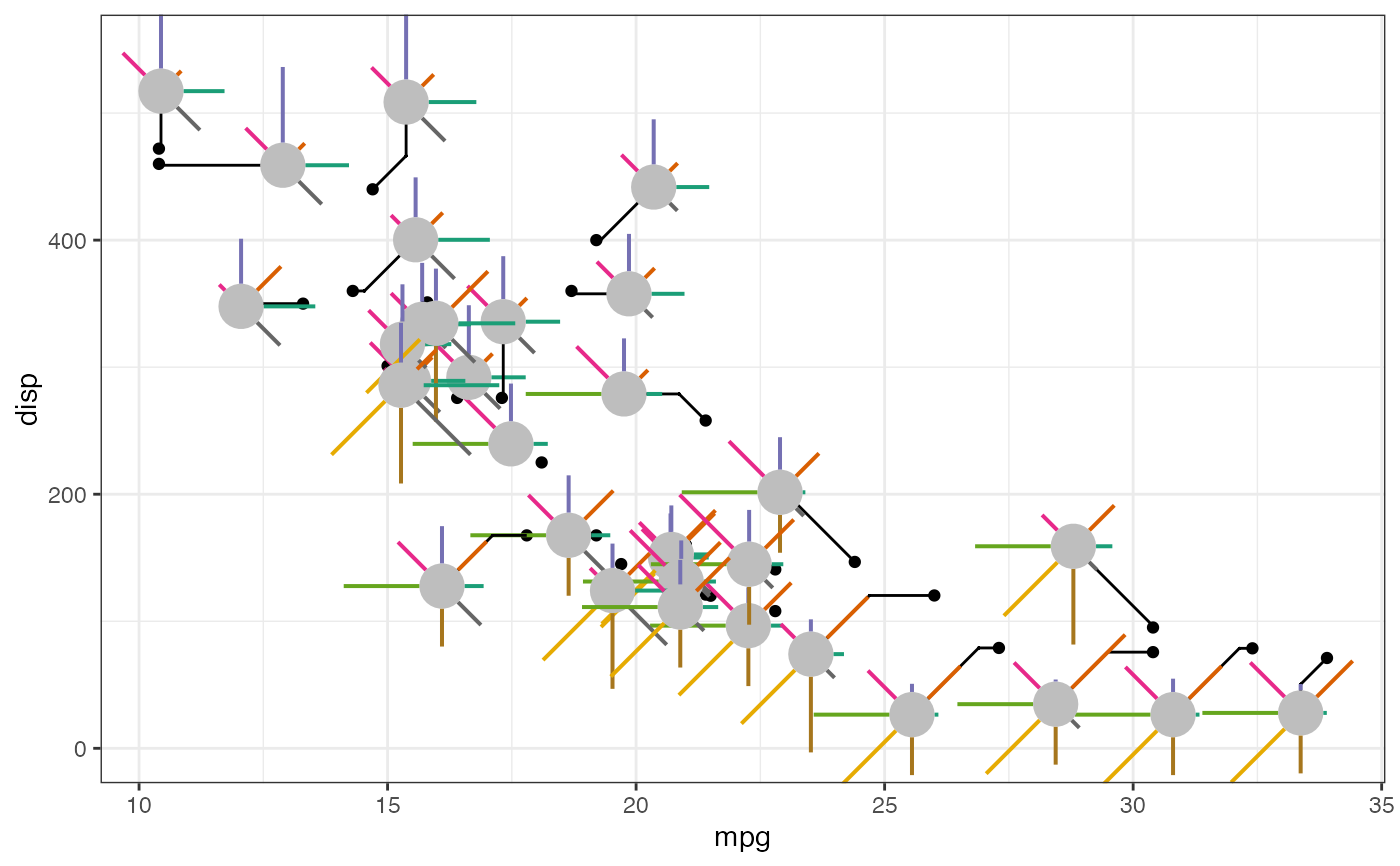
 ggplot(data = mtcars) +
geom_point(aes(x = mpg, y = disp)) +
geom_metroglyph(aes(x = mpg, y = disp),
cols = zs, circle.size = 3,
linewidth.circle = 0, linewidth.ray = 2,
colour.circle = "transparent", fill = "gray",
colour.ray = RColorBrewer::brewer.pal(8, "Dark2"),
size = 10, alpha = 1, repel = TRUE) +
ylim(c(-0, 550))
#> Warning: 11 glyphs have too many overlaps.
#> Consider increasing "max.overlaps"
ggplot(data = mtcars) +
geom_point(aes(x = mpg, y = disp)) +
geom_metroglyph(aes(x = mpg, y = disp),
cols = zs, circle.size = 3,
linewidth.circle = 0, linewidth.ray = 2,
colour.circle = "transparent", fill = "gray",
colour.ray = RColorBrewer::brewer.pal(8, "Dark2"),
size = 10, alpha = 1, repel = TRUE) +
ylim(c(-0, 550))
#> Warning: 11 glyphs have too many overlaps.
#> Consider increasing "max.overlaps"
 #~~~~~~~~~~~~~~~~~~~~~~~~~~~~~~~~~~~~~~~~~~~~~~~~~~~~~~~~~~~~~~~~~~~~~~~~~~~~
# With grid points ----
#~~~~~~~~~~~~~~~~~~~~~~~~~~~~~~~~~~~~~~~~~~~~~~~~~~~~~~~~~~~~~~~~~~~~~~~~~~~~
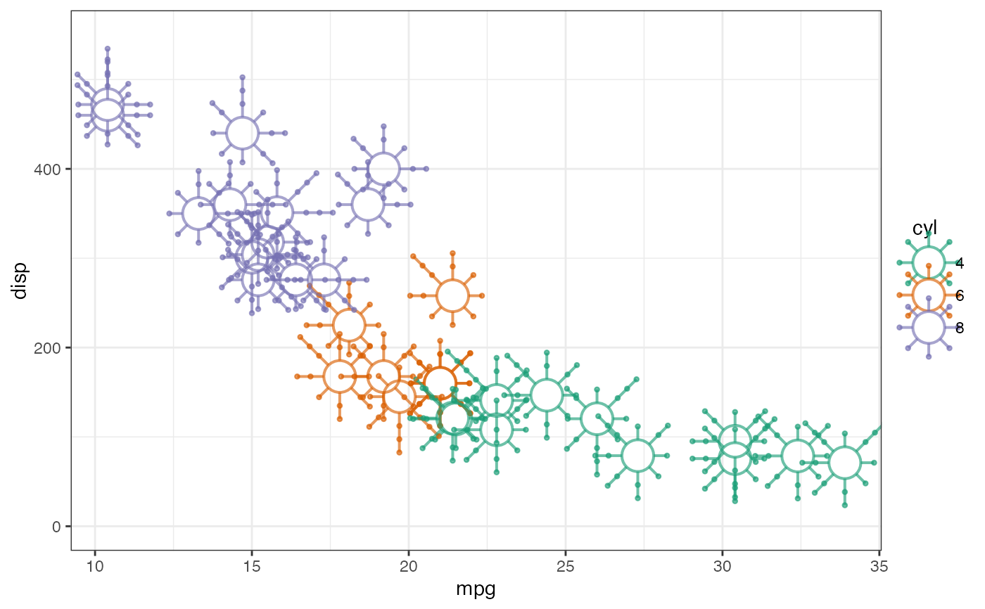
ggplot(data = mtcars_fct) +
geom_metroglyph(aes(x = mpg, y = disp, colour = cyl),
cols = zs, circle.size = 3, colour.ray = NULL,
linewidth.circle = 2, linewidth.ray = 2,
size = 2.5, alpha = 0.8,
draw.grid = TRUE, grid.point.size = 5) +
ylim(c(-0, 550))
#~~~~~~~~~~~~~~~~~~~~~~~~~~~~~~~~~~~~~~~~~~~~~~~~~~~~~~~~~~~~~~~~~~~~~~~~~~~~
# With grid points ----
#~~~~~~~~~~~~~~~~~~~~~~~~~~~~~~~~~~~~~~~~~~~~~~~~~~~~~~~~~~~~~~~~~~~~~~~~~~~~
ggplot(data = mtcars_fct) +
geom_metroglyph(aes(x = mpg, y = disp, colour = cyl),
cols = zs, circle.size = 3, colour.ray = NULL,
linewidth.circle = 2, linewidth.ray = 2,
size = 2.5, alpha = 0.8,
draw.grid = TRUE, grid.point.size = 5) +
ylim(c(-0, 550))
 ggplot(data = mtcars_fct) +
geom_metroglyph(aes(x = mpg, y = disp, fill = cyl),
cols = zs, circle.size = 3, colour.ray = NULL,
linewidth.circle = 2, linewidth.ray = 2,
size = 2.5, alpha = 0.8,
draw.grid = TRUE, grid.point.size = 5) +
ylim(c(-0, 550))
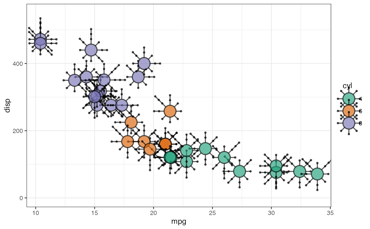
ggplot(data = mtcars_fct) +
geom_metroglyph(aes(x = mpg, y = disp, fill = cyl),
cols = zs, circle.size = 3, colour.ray = NULL,
linewidth.circle = 2, linewidth.ray = 2,
size = 2.5, alpha = 0.8,
draw.grid = TRUE, grid.point.size = 5) +
ylim(c(-0, 550))
 ggplot(data = mtcars_fct) +
geom_metroglyph(aes(x = mpg, y = disp),
cols = zs, circle.size = 3,
linewidth.circle = 0, linewidth.ray = 2,
colour.circle = "transparent", fill = "gray",
colour.ray = RColorBrewer::brewer.pal(8, "Dark2"),
size = 2.5, alpha = 0.8,
draw.grid = TRUE, grid.point.size = 5) +
ylim(c(-0, 550))
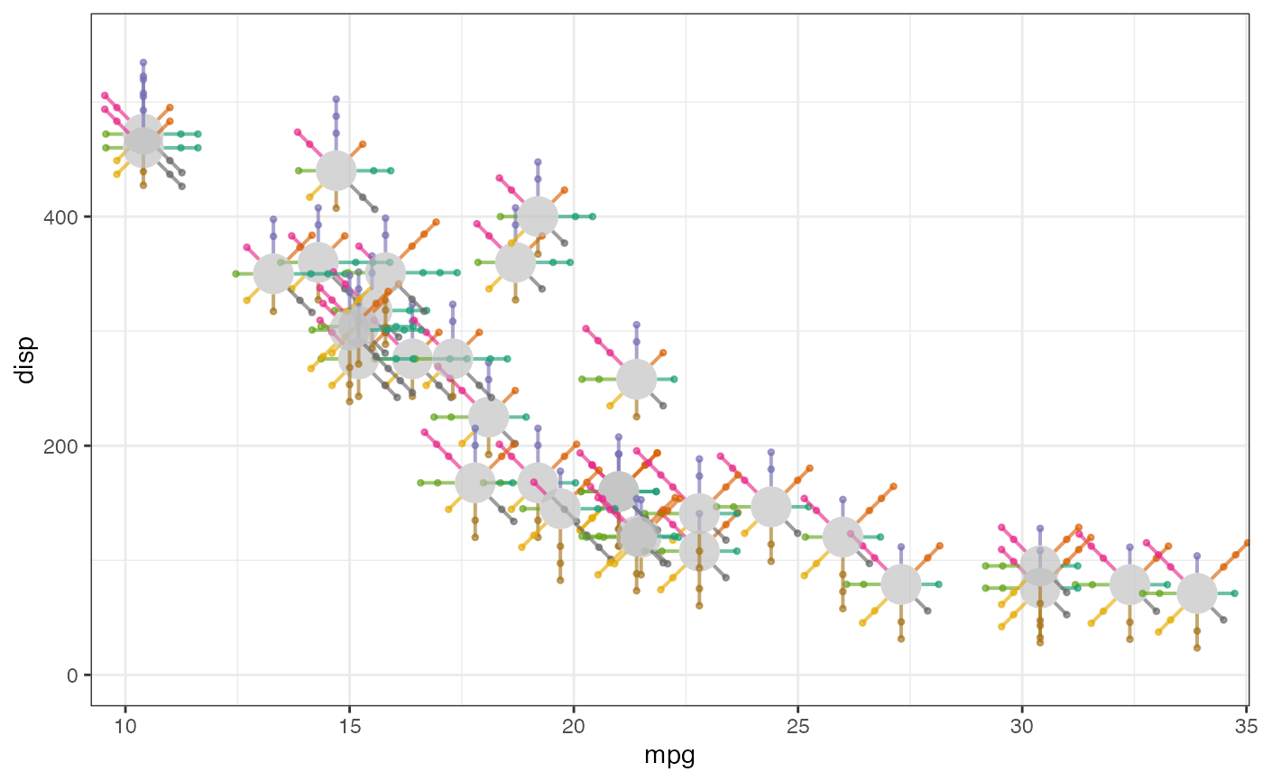
ggplot(data = mtcars_fct) +
geom_metroglyph(aes(x = mpg, y = disp),
cols = zs, circle.size = 3,
linewidth.circle = 0, linewidth.ray = 2,
colour.circle = "transparent", fill = "gray",
colour.ray = RColorBrewer::brewer.pal(8, "Dark2"),
size = 2.5, alpha = 0.8,
draw.grid = TRUE, grid.point.size = 5) +
ylim(c(-0, 550))
 #~~~~~~~~~~~~~~~~~~~~~~~~~~~~~~~~~~~~~~~~~~~~~~~~~~~~~~~~~~~~~~~~~~~~~~~~~~~~
# Legend options ----
#~~~~~~~~~~~~~~~~~~~~~~~~~~~~~~~~~~~~~~~~~~~~~~~~~~~~~~~~~~~~~~~~~~~~~~~~~~~~
# Default legend/guide
ggplot(data = mtcars) +
geom_point(aes(x = mpg, y = disp, colour = cyl)) +
geom_metroglyph(aes(x = mpg, y = disp, colour = cyl),
cols = zs, circle.size = 2, colour.ray = NULL,
linewidth.circle = 2, linewidth.ray = 2,
size = 5, alpha = 1, repel = TRUE) +
ylim(c(-0, 550))
#~~~~~~~~~~~~~~~~~~~~~~~~~~~~~~~~~~~~~~~~~~~~~~~~~~~~~~~~~~~~~~~~~~~~~~~~~~~~
# Legend options ----
#~~~~~~~~~~~~~~~~~~~~~~~~~~~~~~~~~~~~~~~~~~~~~~~~~~~~~~~~~~~~~~~~~~~~~~~~~~~~
# Default legend/guide
ggplot(data = mtcars) +
geom_point(aes(x = mpg, y = disp, colour = cyl)) +
geom_metroglyph(aes(x = mpg, y = disp, colour = cyl),
cols = zs, circle.size = 2, colour.ray = NULL,
linewidth.circle = 2, linewidth.ray = 2,
size = 5, alpha = 1, repel = TRUE) +
ylim(c(-0, 550))
 # Theme modifications for legend
legend_theme <-
theme_bw(base_size = 7.5) +
theme(legend.direction = "vertical",
legend.box = "horizontal",
legend.position = "bottom",
legend.text = element_text(margin = margin(l = 7)),
legend.key.height = unit(1.5, 'lines'))
# Glyph variable-wise legends
ggplot(data = mtcars) +
geom_point(aes(x = mpg, y = disp, colour = cyl)) +
geom_metroglyph(aes(x = mpg, y = disp, colour = cyl),
cols = zs, circle.size = 1, colour.ray = NULL,
linewidth.circle = 2, linewidth.ray = 2,
size = 5, alpha = 1, repel = TRUE) +
ylim(c(-0, 550)) +
scale_z_continuous(z = zs) +
guide_z_order(z = zs, default_aes = "colour") +
legend_theme
# Theme modifications for legend
legend_theme <-
theme_bw(base_size = 7.5) +
theme(legend.direction = "vertical",
legend.box = "horizontal",
legend.position = "bottom",
legend.text = element_text(margin = margin(l = 7)),
legend.key.height = unit(1.5, 'lines'))
# Glyph variable-wise legends
ggplot(data = mtcars) +
geom_point(aes(x = mpg, y = disp, colour = cyl)) +
geom_metroglyph(aes(x = mpg, y = disp, colour = cyl),
cols = zs, circle.size = 1, colour.ray = NULL,
linewidth.circle = 2, linewidth.ray = 2,
size = 5, alpha = 1, repel = TRUE) +
ylim(c(-0, 550)) +
scale_z_continuous(z = zs) +
guide_z_order(z = zs, default_aes = "colour") +
legend_theme
 # Modifying the `legend.glyph.dims`
zavg <- # Scaled average of the variables
apply(mtcars[, zs], 2,
function(x) {
scales::rescale(mean(x),
from = range(x), # same range as in scale_z_continuous
to = c(0, 1))
})
zavg
#> hp drat wt qsec vs am gear carb
#> 0.3345848 0.3855127 0.4357581 0.3986607 0.4375000 0.4062500 0.3437500 0.2589286
ggplot(data = mtcars) +
geom_point(aes(x = mpg, y = disp, colour = cyl)) +
geom_metroglyph(aes(x = mpg, y = disp, colour = cyl),
cols = zs, circle.size = 2, colour.ray = NULL,
linewidth.circle = 2, linewidth.ray = 2,
size = 5, alpha = 1, repel = TRUE) +
ylim(c(-0, 550)) +
xlim(c(8, 35))
#> Warning: 2 glyphs have too many overlaps.
#> Consider increasing "max.overlaps"
# Modifying the `legend.glyph.dims`
zavg <- # Scaled average of the variables
apply(mtcars[, zs], 2,
function(x) {
scales::rescale(mean(x),
from = range(x), # same range as in scale_z_continuous
to = c(0, 1))
})
zavg
#> hp drat wt qsec vs am gear carb
#> 0.3345848 0.3855127 0.4357581 0.3986607 0.4375000 0.4062500 0.3437500 0.2589286
ggplot(data = mtcars) +
geom_point(aes(x = mpg, y = disp, colour = cyl)) +
geom_metroglyph(aes(x = mpg, y = disp, colour = cyl),
cols = zs, circle.size = 2, colour.ray = NULL,
linewidth.circle = 2, linewidth.ray = 2,
size = 5, alpha = 1, repel = TRUE) +
ylim(c(-0, 550)) +
xlim(c(8, 35))
#> Warning: 2 glyphs have too many overlaps.
#> Consider increasing "max.overlaps"
 ggplot(data = mtcars) +
geom_point(aes(x = mpg, y = disp, colour = cyl)) +
geom_metroglyph(aes(x = mpg, y = disp, colour = cyl),
cols = zs, circle.size = 1, colour.ray = NULL,
linewidth.circle = 2, linewidth.ray = 2,
size = 5, alpha = 1, repel = TRUE) +
ylim(c(-0, 550)) +
scale_z_continuous(z = zs) +
guide_z_order(z = zs, default_aes = "colour") +
legend_theme
ggplot(data = mtcars) +
geom_point(aes(x = mpg, y = disp, colour = cyl)) +
geom_metroglyph(aes(x = mpg, y = disp, colour = cyl),
cols = zs, circle.size = 1, colour.ray = NULL,
linewidth.circle = 2, linewidth.ray = 2,
size = 5, alpha = 1, repel = TRUE) +
ylim(c(-0, 550)) +
scale_z_continuous(z = zs) +
guide_z_order(z = zs, default_aes = "colour") +
legend_theme
 # Using custom guide
# metroglyphGrob
guide_metrogrob <- metroglyphGrob(
z = c(0.24, 0.3, 0.8, 1.4, 0.6, 0.33, 0.6, 0.25) * 0.5,
size = 25)
# Add labels to metroglyphGrob
guide_metrogrob <-
addlabel.glyphGrob(grob = guide_metrogrob, label = zs,
push = 1, segment = FALSE)
# Another version
guide_metrogrob2 <- metroglyphGrob(
z = rep(0.3, length(zs)),
size = 25)
guide_metrogrob2 <-
addlabel.glyphGrob(grob = guide_metrogrob2, label = zs,
push = 1, segment = FALSE)
ggplot(data = mtcars) +
geom_point(aes(x = mpg, y = disp, colour = cyl)) +
geom_metroglyph(aes(x = mpg, y = disp, colour = cyl),
cols = zs, circle.size = 1, colour.ray = NULL,
linewidth.circle = 2, linewidth.ray = 2,
size = 5, alpha = 1, repel = TRUE) +
ylim(c(-0, 550)) +
guides(colour = guide_legend(order = 1, position = "right"),
custom = guide_custom(guide_metrogrob,
width = unit(0.1, "npc"),
height = unit(0.1, "npc"),
position = "bottom",
theme = theme(legend.margin = margin(t = 40, b = 30))))
# Using custom guide
# metroglyphGrob
guide_metrogrob <- metroglyphGrob(
z = c(0.24, 0.3, 0.8, 1.4, 0.6, 0.33, 0.6, 0.25) * 0.5,
size = 25)
# Add labels to metroglyphGrob
guide_metrogrob <-
addlabel.glyphGrob(grob = guide_metrogrob, label = zs,
push = 1, segment = FALSE)
# Another version
guide_metrogrob2 <- metroglyphGrob(
z = rep(0.3, length(zs)),
size = 25)
guide_metrogrob2 <-
addlabel.glyphGrob(grob = guide_metrogrob2, label = zs,
push = 1, segment = FALSE)
ggplot(data = mtcars) +
geom_point(aes(x = mpg, y = disp, colour = cyl)) +
geom_metroglyph(aes(x = mpg, y = disp, colour = cyl),
cols = zs, circle.size = 1, colour.ray = NULL,
linewidth.circle = 2, linewidth.ray = 2,
size = 5, alpha = 1, repel = TRUE) +
ylim(c(-0, 550)) +
guides(colour = guide_legend(order = 1, position = "right"),
custom = guide_custom(guide_metrogrob,
width = unit(0.1, "npc"),
height = unit(0.1, "npc"),
position = "bottom",
theme = theme(legend.margin = margin(t = 40, b = 30))))
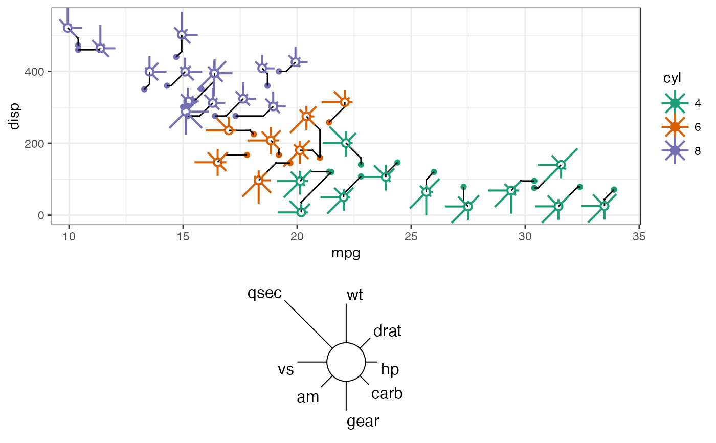 ggplot(data = mtcars) +
geom_point(aes(x = mpg, y = disp, colour = cyl)) +
geom_metroglyph(aes(x = mpg, y = disp, colour = cyl),
cols = zs, circle.size = 1, colour.ray = NULL,
linewidth.circle = 2, linewidth.ray = 2,
size = 5, alpha = 1, repel = TRUE) +
ylim(c(-0, 550)) +
guides(colour = guide_legend(order = 1, position = "right"),
custom = guide_custom(guide_metrogrob2,
width = unit(0.1, "npc"),
height = unit(0.1, "npc"),
position = "bottom",
theme = theme(legend.margin = margin(t = 30, b = 30))))
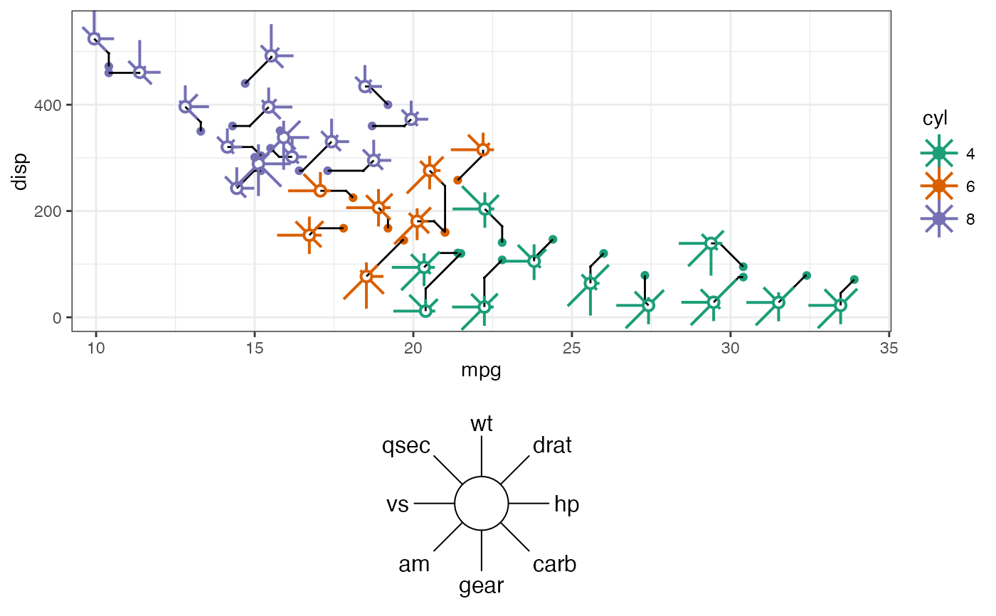
ggplot(data = mtcars) +
geom_point(aes(x = mpg, y = disp, colour = cyl)) +
geom_metroglyph(aes(x = mpg, y = disp, colour = cyl),
cols = zs, circle.size = 1, colour.ray = NULL,
linewidth.circle = 2, linewidth.ray = 2,
size = 5, alpha = 1, repel = TRUE) +
ylim(c(-0, 550)) +
guides(colour = guide_legend(order = 1, position = "right"),
custom = guide_custom(guide_metrogrob2,
width = unit(0.1, "npc"),
height = unit(0.1, "npc"),
position = "bottom",
theme = theme(legend.margin = margin(t = 30, b = 30))))
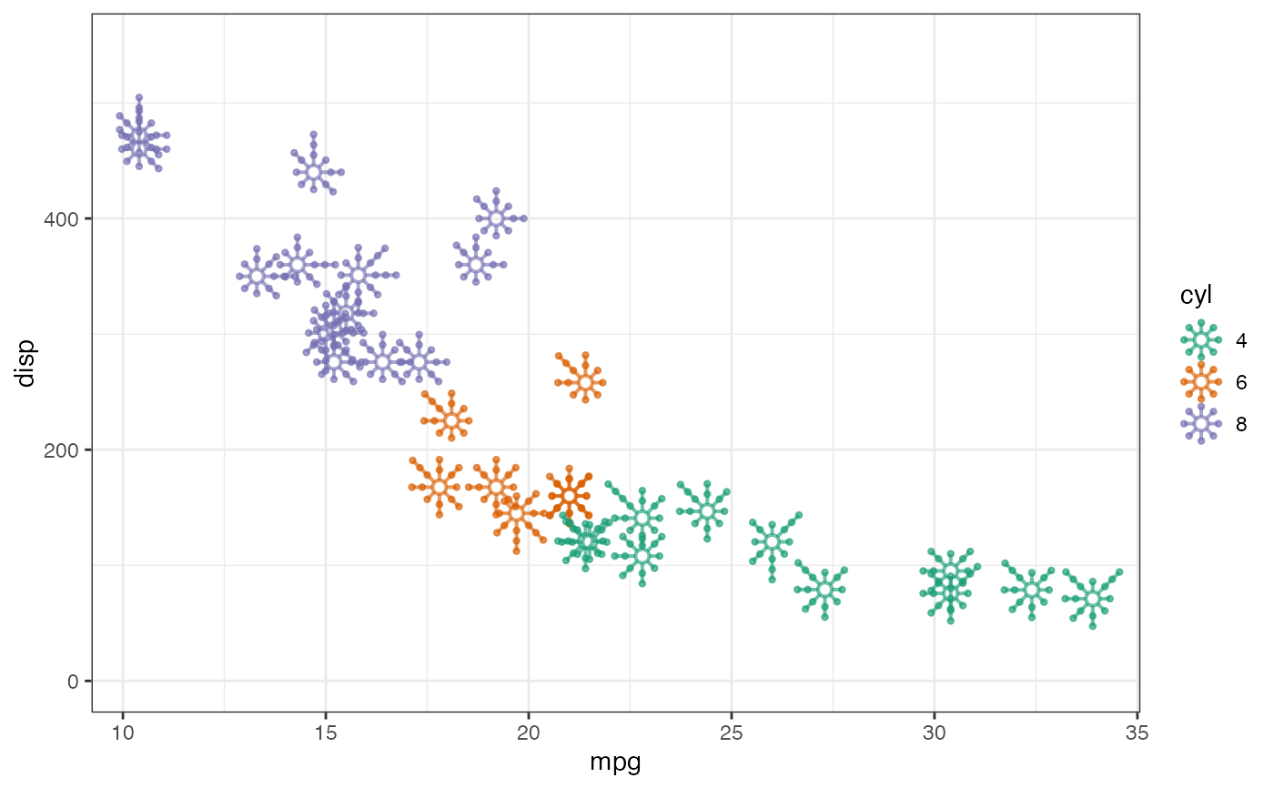
 # Legend in plots with grid points
z_grid <- c(hp = 3, drat = 3, wt = 2,
qsec = 2, vs = 3, am = 4,
gear = 2, carb = 3)
ggplot(data = mtcars_fct) +
geom_metroglyph(aes(x = mpg, y = disp, colour = cyl),
cols = zs, circle.size = 1, colour.ray = NULL,
linewidth.circle = 2, linewidth.ray = 2,
size = 1.5, alpha = 0.8,
draw.grid = TRUE, grid.point.size = 5) +
ylim(c(-0, 550))
# Legend in plots with grid points
z_grid <- c(hp = 3, drat = 3, wt = 2,
qsec = 2, vs = 3, am = 4,
gear = 2, carb = 3)
ggplot(data = mtcars_fct) +
geom_metroglyph(aes(x = mpg, y = disp, colour = cyl),
cols = zs, circle.size = 1, colour.ray = NULL,
linewidth.circle = 2, linewidth.ray = 2,
size = 1.5, alpha = 0.8,
draw.grid = TRUE, grid.point.size = 5) +
ylim(c(-0, 550))
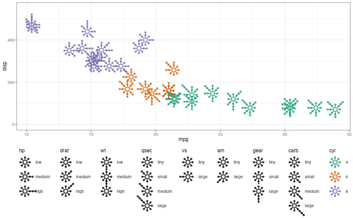
 ggplot(data = mtcars_fct) +
geom_metroglyph(aes(x = mpg, y = disp, colour = cyl),
cols = zs, circle.size = 1, colour.ray = NULL,
linewidth.circle = 2, linewidth.ray = 2,
size = 1.5, alpha = 0.8,
draw.grid = TRUE, grid.point.size = 5) +
ylim(c(-0, 550)) +
scale_z_discrete(z = zs) +
guide_z_order(z = zs, default_aes = "fill") +
legend_theme
ggplot(data = mtcars_fct) +
geom_metroglyph(aes(x = mpg, y = disp, colour = cyl),
cols = zs, circle.size = 1, colour.ray = NULL,
linewidth.circle = 2, linewidth.ray = 2,
size = 1.5, alpha = 0.8,
draw.grid = TRUE, grid.point.size = 5) +
ylim(c(-0, 550)) +
scale_z_discrete(z = zs) +
guide_z_order(z = zs, default_aes = "fill") +
legend_theme
 ggplot(data = mtcars_fct) +
geom_metroglyph(aes(x = mpg, y = disp, colour = cyl),
cols = zs, circle.size = 1, colour.ray = NULL,
linewidth.circle = 2, linewidth.ray = 2,
size = 1.5, alpha = 0.8,
draw.grid = TRUE, grid.point.size = 5,
legend.glyph.dims = z_grid) +
ylim(c(-0, 550))
ggplot(data = mtcars_fct) +
geom_metroglyph(aes(x = mpg, y = disp, colour = cyl),
cols = zs, circle.size = 1, colour.ray = NULL,
linewidth.circle = 2, linewidth.ray = 2,
size = 1.5, alpha = 0.8,
draw.grid = TRUE, grid.point.size = 5,
legend.glyph.dims = z_grid) +
ylim(c(-0, 550))
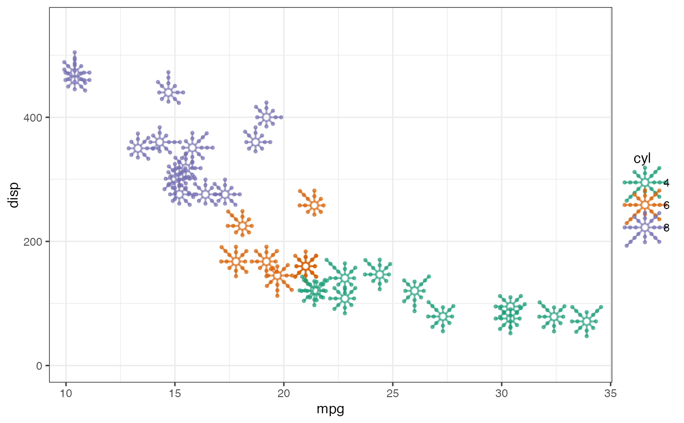 ggplot(data = mtcars_fct) +
geom_metroglyph(aes(x = mpg, y = disp, colour = cyl),
cols = zs, circle.size = 1, colour.ray = NULL,
linewidth.circle = 2, linewidth.ray = 2,
size = 1.5, alpha = 0.8,
draw.grid = TRUE, grid.point.size = 5,
legend.glyph.dims = z_grid) +
ylim(c(-0, 550)) +
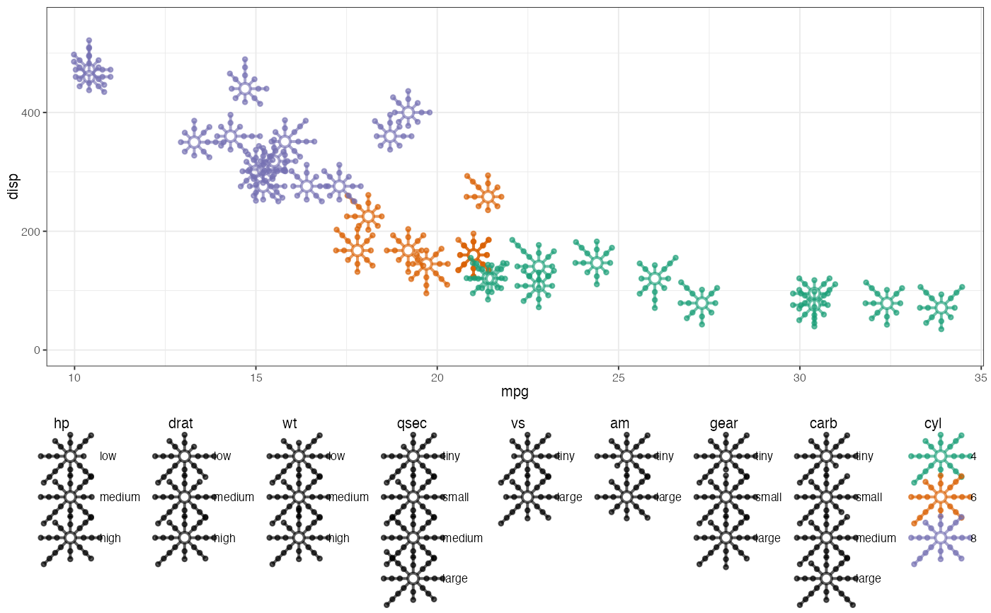
scale_z_discrete(z = zs) +
guide_z_order(z = zs, default_aes = "fill") +
legend_theme
ggplot(data = mtcars_fct) +
geom_metroglyph(aes(x = mpg, y = disp, colour = cyl),
cols = zs, circle.size = 1, colour.ray = NULL,
linewidth.circle = 2, linewidth.ray = 2,
size = 1.5, alpha = 0.8,
draw.grid = TRUE, grid.point.size = 5,
legend.glyph.dims = z_grid) +
ylim(c(-0, 550)) +
scale_z_discrete(z = zs) +
guide_z_order(z = zs, default_aes = "fill") +
legend_theme
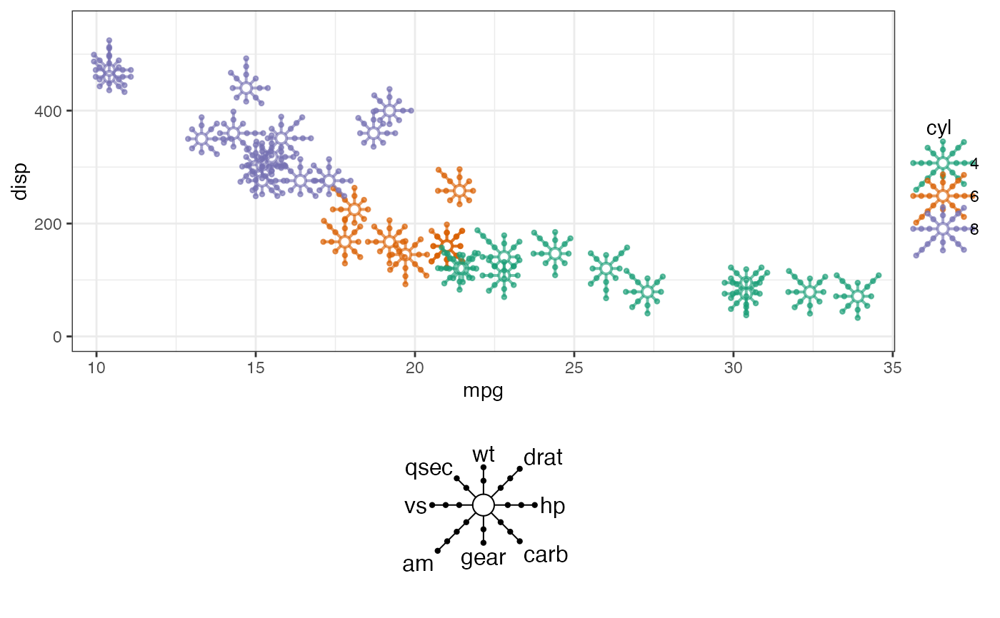
 # metroglyphGrob with grid levels
z_grid_levels <- lapply(z_grid, function(x) 1:x)
guide_metrogrob_grid <-
metroglyphGrob(z = z_grid,
size = 2.5, draw.grid = TRUE, circle.size = 2,
grid.levels = z_grid_levels,
grid.point.size = 0.1)
guide_metrogrob_grid <-
addlabel.glyphGrob(grob = guide_metrogrob_grid, label = zs,
push = 1, segment = FALSE)
# Another version
guide_metrogrob_grid2 <-
metroglyphGrob(z = rep(3, length(z_grid)),
size = 2.5, draw.grid = TRUE, circle.size = 2,
grid.levels = replicate(8, 1:3,
simplify = FALSE),
grid.point.size = 0.1)
guide_metrogrob_grid2 <-
addlabel.glyphGrob(grob = guide_metrogrob_grid2, label = zs,
push = 1, segment = FALSE)
ggplot(data = mtcars_fct) +
geom_metroglyph(aes(x = mpg, y = disp, colour = cyl),
cols = zs, circle.size = 1, colour.ray = NULL,
linewidth.circle = 2, linewidth.ray = 2,
size = 1.5, alpha = 0.8,
draw.grid = TRUE, grid.point.size = 5,
legend.glyph.dims = z_grid) +
ylim(c(-0, 550)) +
guides(fill = guide_legend(order = 1, position = "right"),
custom = guide_custom(guide_metrogrob_grid,
width = unit(0.1, "npc"),
height = unit(0.1, "npc"),
position = "bottom",
theme = theme(legend.margin = margin(t = 20, b = 30))))
# metroglyphGrob with grid levels
z_grid_levels <- lapply(z_grid, function(x) 1:x)
guide_metrogrob_grid <-
metroglyphGrob(z = z_grid,
size = 2.5, draw.grid = TRUE, circle.size = 2,
grid.levels = z_grid_levels,
grid.point.size = 0.1)
guide_metrogrob_grid <-
addlabel.glyphGrob(grob = guide_metrogrob_grid, label = zs,
push = 1, segment = FALSE)
# Another version
guide_metrogrob_grid2 <-
metroglyphGrob(z = rep(3, length(z_grid)),
size = 2.5, draw.grid = TRUE, circle.size = 2,
grid.levels = replicate(8, 1:3,
simplify = FALSE),
grid.point.size = 0.1)
guide_metrogrob_grid2 <-
addlabel.glyphGrob(grob = guide_metrogrob_grid2, label = zs,
push = 1, segment = FALSE)
ggplot(data = mtcars_fct) +
geom_metroglyph(aes(x = mpg, y = disp, colour = cyl),
cols = zs, circle.size = 1, colour.ray = NULL,
linewidth.circle = 2, linewidth.ray = 2,
size = 1.5, alpha = 0.8,
draw.grid = TRUE, grid.point.size = 5,
legend.glyph.dims = z_grid) +
ylim(c(-0, 550)) +
guides(fill = guide_legend(order = 1, position = "right"),
custom = guide_custom(guide_metrogrob_grid,
width = unit(0.1, "npc"),
height = unit(0.1, "npc"),
position = "bottom",
theme = theme(legend.margin = margin(t = 20, b = 30))))
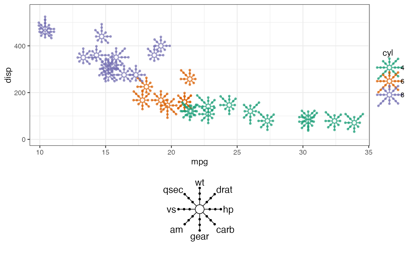
 ggplot(data = mtcars_fct) +
geom_metroglyph(aes(x = mpg, y = disp, colour = cyl),
cols = zs, circle.size = 1, colour.ray = NULL,
linewidth.circle = 2, linewidth.ray = 2,
size = 1.5, alpha = 0.8,
draw.grid = TRUE, grid.point.size = 5,
legend.glyph.dims = z_grid) +
ylim(c(-0, 550)) +
guides(fill = guide_legend(order = 1, position = "right"),
custom = guide_custom(guide_metrogrob_grid2,
width = unit(0.1, "npc"),
height = unit(0.1, "npc"),
position = "bottom",
theme = theme(legend.margin = margin(t = 20, b = 30))))
ggplot(data = mtcars_fct) +
geom_metroglyph(aes(x = mpg, y = disp, colour = cyl),
cols = zs, circle.size = 1, colour.ray = NULL,
linewidth.circle = 2, linewidth.ray = 2,
size = 1.5, alpha = 0.8,
draw.grid = TRUE, grid.point.size = 5,
legend.glyph.dims = z_grid) +
ylim(c(-0, 550)) +
guides(fill = guide_legend(order = 1, position = "right"),
custom = guide_custom(guide_metrogrob_grid2,
width = unit(0.1, "npc"),
height = unit(0.1, "npc"),
position = "bottom",
theme = theme(legend.margin = margin(t = 20, b = 30))))
 # }
# }